Ccy:别再只画折线图了,用 Python 做一张“模型鲁棒性相变图”

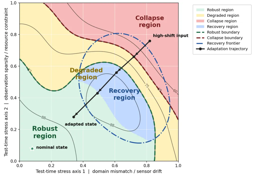
import numpy as npimport matplotlib.pyplot as pltfrom matplotlib.colors import ListedColormap, BoundaryNormfrom matplotlib.patches import Patchnp.random.seed(7)x = np.linspace(0, 1, 260)y = np.linspace(0, 1, 260)X, Y = np.meshgrid(x, y)raw_task_perf = (    92    - 18 * X**1.6    - 22 * Y**1.8    - 35 * (X * Y)**1.2    + 2.5 * np.sin(3 * np.pi * X) * np.cos(2 * np.pi * Y))adaptation_gain = (    18 * np.exp(-((X - 0.62)**2 / 0.055 + (Y - 0.52)**2 / 0.075))    + 10 * np.exp(-((X - 0.78)**2 / 0.035 + (Y - 0.30)**2 / 0.045)))adapted_task_perf = raw_task_perf + adaptation_gainadapted_task_perf = np.clip(adapted_task_perf, 35, 94)phase = np.zeros_like(adapted_task_perf, dtype=int)phase[adapted_task_perf < 68] = 2phase[(adapted_task_perf >= 68) & (adapted_task_perf < 82)] = 1phase[adapted_task_perf >= 82] = 0recovery_mask = (    (raw_task_perf < 78)    & (adapted_task_perf >= 82)    & (adaptation_gain > 6))phase[recovery_mask] = 3plt.rcParams["font.family"] = "DejaVu Sans"plt.rcParams["axes.unicode_minus"] = Falsefig, ax = plt.subplots(figsize=(10.8, 7.2), dpi=150)phase_colors = [    "#D7F2E3",  # Robust    "#FFF1B8",  # Degraded    "#F6B6B6",  # Collapse    "#BFD7FF",  # Recovery]cmap = ListedColormap(phase_colors)norm = BoundaryNorm([-0.5, 0.5, 1.5, 2.5, 3.5], cmap.N)ax.pcolormesh(X, Y, phase, cmap=cmap, norm=norm, shading="auto", alpha=0.96)contours = ax.contour(    X, Y, adapted_task_perf,    levels=[60, 68, 75, 82, 88],    colors="k",    linewidths=[1.0, 1.8, 1.0, 1.8, 1.0],    alpha=0.62)ax.clabel(contours, inline=True, fontsize=9, fmt="%d")ax.contour(    X, Y, adapted_task_perf,    levels=[68],    colors="#7A1F1F",    linewidths=2.8,    linestyles="--")ax.contour(    X, Y, adapted_task_perf,    levels=[82],    colors="#1C6B43",    linewidths=2.8,    linestyles="--")ax.contour(    X, Y, adaptation_gain,    levels=[6],    colors="#2356A4",    linewidths=2.4,    linestyles="-.")trajectory = np.array([    [0.82, 0.76],    [0.72, 0.66],    [0.61, 0.56],    [0.49, 0.43],    [0.34, 0.28],])ax.plot(    trajectory[:, 0],    trajectory[:, 1],    color="#222222",    linewidth=2.4,    marker="o",    markersize=5.5,    zorder=5)for i in range(len(trajectory) - 1):    ax.annotate(        "",        xy=trajectory[i + 1],        xytext=trajectory[i],        arrowprops=dict(            arrowstyle="->",            color="#222222",            lw=2.0,            shrinkA=5,            shrinkB=5        ),        zorder=6    )ax.text(    trajectory[0, 0] + 0.02,    trajectory[0, 1] + 0.025,    "high-shift input",    fontsize=10,    weight="bold")ax.text(    trajectory[-1, 0] - 0.055,    trajectory[-1, 1] - 0.055,    "adapted state",    fontsize=10,    weight="bold")ax.scatter(    [0.08], [0.08],    s=170,    marker="*",    color="#1B7F4C",    edgecolor="white",    linewidth=1.4,    zorder=7)ax.text(    0.105, 0.085,    "nominal state",    fontsize=10,    weight="bold",    va="center")ax.text(    0.16, 0.18,    "Robust\nregion",    fontsize=16,    weight="bold",    color="#145A32",    ha="center",    va="center")ax.text(    0.42, 0.55,    "Degraded\nregion",    fontsize=15,    weight="bold",    color="#8A6D00",    ha="center",    va="center")ax.text(    0.82, 0.88,    "Collapse\nregion",    fontsize=15,    weight="bold",    color="#7A1F1F",    ha="center",    va="center")ax.text(    0.66, 0.42,    "Recovery\nregion",    fontsize=15,    weight="bold",    color="#1F4E8C",    ha="center",    va="center")legend_elements = [    Patch(facecolor=phase_colors[0], edgecolor="none", label="Robust region"),    Patch(facecolor=phase_colors[1], edgecolor="none", label="Degraded region"),    Patch(facecolor=phase_colors[2], edgecolor="none", label="Collapse region"),    Patch(facecolor=phase_colors[3], edgecolor="none", label="Recovery region"),]line_legend = [    plt.Line2D([0], [0], color="#1C6B43", lw=2.6, ls="--", label="Robust boundary"),    plt.Line2D([0], [0], color="#7A1F1F", lw=2.6, ls="--", label="Collapse boundary"),    plt.Line2D([0], [0], color="#2356A4", lw=2.4, ls="-.", label="Recovery frontier"),    plt.Line2D([0], [0], color="#222222", lw=2.4, marker="o", label="Adaptation trajectory"),]ax.legend(    handles=legend_elements + line_legend,    loc="upper left",    bbox_to_anchor=(1.08, 1.0),    frameon=True,    framealpha=0.94,    fontsize=9.5,    borderpad=0.9)ax.set_title(    "Robustness Phase Diagram: Performance Phase Transition under Compound Test-Time Shifts",    fontsize=15,    weight="bold",    pad=14)ax.set_xlabel("Test-time stress axis 1  |  domain mismatch / sensor drift", fontsize=11)ax.set_ylabel("Test-time stress axis 2  |  observation sparsity / resource constraint", fontsize=11)ax.set_xlim(0, 1)ax.set_ylim(0, 1)ax.set_xticks(np.linspace(0, 1, 6))ax.set_yticks(np.linspace(0, 1, 6))ax.grid(    color="white",    linestyle="-",    linewidth=0.8,    alpha=0.65)ax.set_aspect("equal", adjustable="box")ax.text(    0.02, -0.12,    "Contours indicate adapted downstream task performance. "    "Dashed lines mark phase-transition boundaries.",    transform=ax.transAxes,    fontsize=9.5,    color="#444444")plt.tight_layout(rect=[0, 0.03, 0.78, 1])plt.show()