Python | 绘制黑底图片

写在前面

最近汉堡的天气热得出奇，本来就因为论文第三章该做什么而烦躁，现在更觉得心情被热浪也放大了。

目前的状态有点卡在一个尴尬的分界线上：一方面，我仍然享受待在熟悉的波动研究舒适区里，因为这个方向相对熟悉，也更容易形成逻辑；另一方面，我又想跨出去，尝试一些更不一样、更落地、甚至更偏应用的问题。但现实限制也很明显。

• 考虑到 ICON 当前的模拟能力，有些 idea 并不太容易真正落地；如果做区域分析，误差又会比较大，很多地方都受限。结果就变成了：既不想完全停留在理论层面，又不得不在各种限制里“鸡蛋里挑骨头”，努力找出一点有新意、也相对可行的东西。

昨天组会简单汇报了一下几个可能的思路。好在这次至少把当前的想法比较清楚地讲给了外导，也得到了初步认可。但真正开始处理 MCSs 的时候，又发现里面有各种各样的问题：数据、追踪、阈值、解释逻辑，好像每一步都没有想象中顺畅。

今天看邮件，连老外都建议大家可以居家弹性办公。可惜家里没有空调，待在家里也像蒸拿房一样，似乎并没有比办公室舒服多少。

所以这一周还是先以看文献和写代码交替推进为主。最近也明显感觉到，AI 用得越熟练，反而越容易让人变懒，甚至代码能力也有点下降。很多时候直接让 AI 帮忙写，短期效率是提高了，但长期看可能会削弱自己手写代码、独立 debug 和组织思路的能力。甚至有时候越依赖，脑子越像被雾蒙住一样。所以接下来还是有必要多自己手写代码，哪怕慢一点，也能重新把思路和能力找回来。

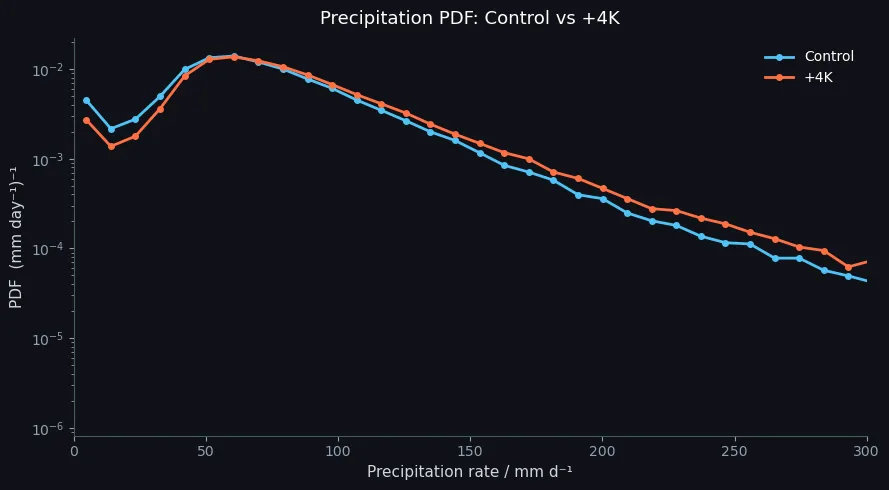
极端降水概率分布

随便两组对比数据的降水序列，然后进行比较。得到以下结果，为了回报，可以将PPT的底图调整为黑色，更搭配PPT或者其他展示的背景。

python

fig, ax = plt.subplots(figsize=(9, 5))
fig.patch.set_facecolor('#0f1117')
ax.set_facecolor('#0f1117')

CNTL_COLOR = '#4fc3f7'
P4K_COLOR  = '#ff7043'

ax.plot(bin_centers, pdf_cntl, color=CNTL_COLOR, lw=2, marker='o', ms=4, label='Control', zorder=3)
ax.plot(bin_centers, pdf_p4k,  color=P4K_COLOR,  lw=2, marker='o', ms=4, label='+4K',     zorder=3)

ax.set_yscale('log')

ax.set_xscale('log')
ax.set_xlabel('Precipitation rate / mm d⁻¹', color='#cfd8dc', fontsize=11)
ax.set_ylabel('PDF  (mm day⁻¹)⁻¹',              color='#cfd8dc', fontsize=11)
ax.set_title('Precipitation PDF: Control vs +4K', color='white', fontsize=13, pad=10)
ax.set_xlim(0, 300)

ax.tick_params(colors='#90a4ae', which='both')
ax.spines[['top', 'right']].set_visible(False)
for sp in ['bottom', 'left']:
    ax.spines[sp].set_color('#455a64')

ax.legend(framealpha=0.25, facecolor='#263238',frameon=False,
          edgecolor='#546e7a', labelcolor='white', fontsize=10)

plt.tight_layout()

plt.show()

通过一个转化的方法

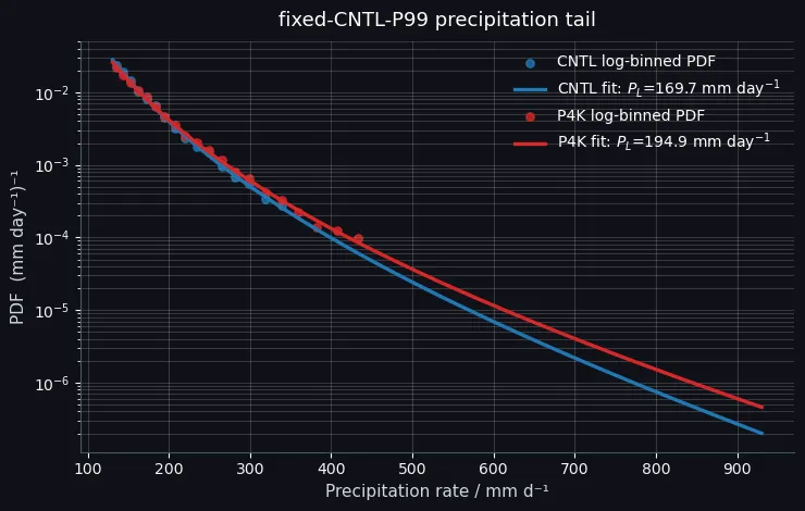
曲线往右下降得越慢，说明高强度降水出现的相对概率越高。 图里 P4K 的红色拟合线在高降水强度区间明显高于 CNTL，说明：增暖后，降水尾部变“更厚”了，更强降水事件的概率相对增加。

from scipy.integrate import quad

TAIL_PERCENTILE = 90# shared, absolute P_min for a like-for-like tail comparison
N_LOG_BINS, MIN_BIN_COUNT, N_BOOTSTRAP = 32, 20, 250
pooled_vals = np.concatenate([cntl_vals, p4k_vals])
P_min = np.percentile(pooled_vals, TAIL_PERCENTILE)
P_max = pooled_vals.max() * (1 + 1e-10)
tail_bins = np.geomspace(P_min, P_max, N_LOG_BINS + 1)

deffit_precipitation_tail(values, bins=tail_bins, min_bin_count=MIN_BIN_COUNT):
"""Log-bin fit of tau and P_L for the conditional P >= P_min PDF."""
    tail = np.asarray(values)[np.asarray(values) >= bins[0]]
    counts, _ = np.histogram(tail, bins=bins)
    pdf, _ = np.histogram(tail, bins=bins, density=True)
    centers = np.sqrt(bins[:-1] * bins[1:])
    use = (counts >= min_bin_count) & np.isfinite(pdf) & (pdf > 0)
if use.sum() < 3:
raise ValueError('Too few populated tail bins for a three-parameter fit.')

# Intercept, -tau, and -1/P_L: identical linear form to the reference demo.
    X = np.column_stack([np.ones(use.sum()), np.log(centers[use]), centers[use]])
    log_c_fit, minus_tau, minus_inv_PL = np.linalg.lstsq(X, np.log(pdf[use]), rcond=None)[0]
    tau, P_L = -minus_tau, -1 / minus_inv_PL
ifnot np.isfinite(P_L) or P_L <= 0:
raise ValueError('Non-negative exponential slope: P_L is undefined.')

# c is the factor that normalizes this conditional tail PDF over [P_min, infinity).
    integral, _ = quad(lambda p: p**(-tau) * np.exp(-p / P_L), bins[0], np.inf)
    c = 1 / integral
    fitted = X @ np.array([log_c_fit, minus_tau, minus_inv_PL])
    observed = np.log(pdf[use])
    r_squared = 1 - np.sum((observed - fitted)**2) / np.sum((observed - observed.mean())**2)
return dict(tail=tail, counts=counts, pdf=pdf, centers=centers, use=use,
                tau=tau, P_L=P_L, c=c, r_squared=r_squared)

★

Duan, S. Q., W.-M. Tsai, F. Ahmed, and J. D. Neelin, 2026: Extreme-range precipitation probability across global weather systems. Science ADvAnceS.