python 烟羽模型实现,及三维地图展示

#高斯模型计算exampleData = np.load('exampleData.npz')#打包数据gasConc = exampleData['gasConc']#环境六参中的一个temp = exampleData['temp']#温度pres = exampleData['pres']#压力#z x y的风向ws3z = exampleData['ws3z']ws3x = exampleData['ws3x']ws3y = exampleData['ws3y']#distance = exampleData['distance']distance = np.array((200.0))#距离 是个变量可更改#返回u、v、w、windir风向、windSpeed风速fieldArr = OTA33A.fieldData(gasConc,temp,pres,ws3z,ws3x,ws3y,distance,16.04,'PM2.5')#求出数据的排放率（massRate） 和 方向度（yFitMax）massRate, yFitMax = fieldArr.getEmissionRate(make_plot=True)

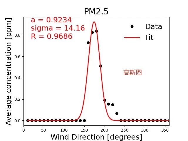
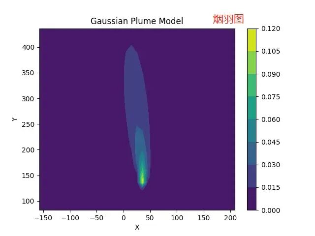
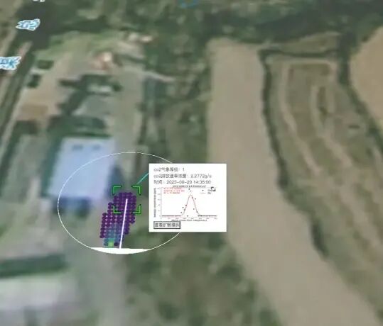
from math import trunc  # 用于截断数字的函数import numpy as np  # 数值计算库from scipy.optimize import curve_fit  # 曲线拟合函数####################    常量定义      ####################R = 0.08205746 # 通用气体常数 [L atm K-1 mol-1]P_stp = 1. # 标准大气压 [atm]T_stp = 298 # 标准温度 [K]def gaussian_func(x,a,sigma,x_0):    """    高斯函数    返回具有适当系数的高斯函数值    :param x: 自变量    :param a: 振幅参数    :param sigma: 标准差参数    :param x_0: 中心位置参数    :return: 高斯函数值    """    return a*np.exp(-((x - x_0)**2)/(2*sigma**2))def stability_class(std_wind,turb,v=False):    """    根据风速标准差和湍流强度确定平均稳定性等级    :param std_wind: 水平风向标准差 [度]    :param turb: 湍流强度    :param v: 是否输出详细信息    :return: 平均稳定性等级    """    # 根据风速标准差确定水平稳定性等级    if std_wind > 27.5:        pg_wind = 1    elif std_wind <=27.5 and std_wind > 23.5:        pg_wind = 2    elif std_wind <=23.5 and std_wind >19.5:        pg_wind = 3    elif std_wind <= 19.5 and std_wind > 15.5:        pg_wind = 4    elif std_wind <= 15.5 and std_wind > 11.5:        pg_wind = 5    elif std_wind <= 11.5 and std_wind > 7.5:        pg_wind = 6    elif std_wind <= 7.50:        pg_wind = 7    if v:        print("Horizontal Stability class = %d "%(pg_wind))    # 根据湍流强度确定垂直稳定性等级    if turb > 0.205:        pg_turb = 1    elif turb <= .205 and turb > 0.180:        pg_turb = 2    elif turb <= 0.180 and turb > 0.155:        pg_turb = 3    elif turb <=0.155 and turb > 0.130:        pg_turb = 4    elif turb <= 0.130 and turb > 0.105:        pg_turb = 5    elif turb <= 0.105 and turb > 0.080:        pg_turb = 6    elif turb <= 0.080:        pg_turb = 7    if v:        print("Vertical Stability class = %d "%(pg_turb))    # 计算最终的平均稳定性等级    final_pg = int(np.ceil(np.mean((pg_wind,pg_turb))))    return final_pgdef sigma_func(I,J,K,dist):    """    用于基于稳定性参数估算sigma_y和sigma_z的函数    :param I: 参数I    :param J: 参数J    :param K: 参数K    :param dist: 距离    :return: 计算结果    """    return np.exp(I + J*np.log(dist) + K*(np.log(dist)**2))def sigma(dist,std_wind=None,turb=None,stab= None,tables=False,v=False):    """    计算排放分布的水平和垂直标准差    七个自定义类别基于Pasquill-Gifford模型的方式：    1 - PG class A    2 - PG classes A and B之间的线性插值    3 - PG class B    4 - PG classes B and C之间的线性插值    5 - PG class C    6 - PG classes C and D之间的线性插值    7 - PG class D    :param dist: 接收器和源之间的距离    :param std_wind: 水平风向标准差 [度]    :param turb: 湍流强度    :param stab: 稳定性等级    :param tables: 是否使用表格    :param v: 是否输出详细信息    :return: sigma_y, sigma_z, 稳定性等级    """    if stab == None:        stab = stability_class(std_wind,turb,v=v)    # 加载水平扩散参数表    file_y = np.load('ota33a/pgtabley.npz')    pgtabley = file_y['data']    sigma_y = pgtabley[trunc(np.round(dist)-1),stab-1]    # 加载垂直扩散参数表    file_y = np.load('ota33a/pgtablez.npz')    pgtablez = file_y['data']    sigma_z = pgtablez[trunc(np.round(dist)-1),stab-1]    return sigma_y,sigma_z,stabdef ppm2gm3(conc,mw,T,P):    """    将以ppm为单位的浓度转换为g/m3单位的浓度    :param conc: 浓度 [ppb]    :param mw: 分子量 [g/mol]    :param T: 温度 [K]    :param P: 压力 [atm]    :return: 浓度 [g/m3]    """    R = 0.08205746 # 通用气体常数 [L atm K-1 mol-1]    mass = conc*mw    V = (1e6*R*T)/(P*1000.)    return mass/Vdef fit_plot(x,y_data,fit,name):    """    绘制实际数据与执行的高斯拟合对比图    :param x: 风向箱    :param y_data: 计算的平均浓度    :param fit: 高斯函数的拟合系数    :param name: 图表标题    :return: 最大拟合值对应的x轴值    """    try:        import matplotlib.pyplot as plt        xAnalytic = np.linspace(x.min(),x.max(),1000)        y_fit = gaussian_func(xAnalytic,fit[0],fit[1],fit[2])        R = np.corrcoef(y_data,gaussian_func(x,fit[0],fit[1],fit[2]))[0,1]        fs=18        fig = plt.figure()        ax = fig.add_subplot(111)        ax.plot(x,y_data,'o',c='k',label='Data',lw=2)        ax.plot(xAnalytic,y_fit,c='r',label='Fit',lw=2)    #画线 可用来确认对高点        ax.set_xlabel('Wind Direction [degrees]',fontsize=fs)        ax.set_ylabel('Average concentration [ppm]',fontsize=fs)        ax.set_title(name,fontsize=fs+2)        ax.set_xlim(0,360)        ax.text(np.diff(ax.get_xlim())*.05+ax.get_xlim()[0],np.diff(ax.get_ylim())*.8+ax.get_ylim()[0],'a = %.4f\nsigma = %.2f\nR = %.4f' % (fit[0],fit[1],R),color='r',fontsize=18)        leg=ax.legend(fontsize=fs)        leg.get_frame().set_alpha(0.)        plt.show()        #plt.savefig("./pic/" + name + ".png", transparent=True, bbox_inches="tight", pad_inches=0)        #找y_fit中的最大值 对应的 x轴方向度数        yFitMax = max(y_fit)        for i in range(len(y_fit)):            if y_fit[i] == yFitMax:                return xAnalytic[i]    except:        print('Your system does not appear to have Matplotlib installed. This is \        required to make a plot')def yamartino_method(wd):    """    使用Yamartino方法计算风向标准差    该方法的更多信息可以在Wikipedia上找到(http://en.wikipedia.org/wiki/Yamartino_method)    或原始论文:    Yamartino, R.J. (1984). "A Comparison of Several "Single-Pass" Estimators of the Standard Deviation of    Wind Direction". Journal of Climate and Applied Meteorology 23 (9): 1362-1366.    :param wd: 风向数组 [度]    :return: 风向标准差 [度]    """    n = float(len(wd))    sa = np.mean(np.sin(wd*np.pi/180))    ca = np.mean(np.cos(wd*np.pi/180))    epsilon = np.sqrt(1 - (sa**2 + ca**2))    std_wd = np.sqrt(n/(n-1))*np.arcsin(epsilon)*(1 + (2./np.sqrt(3) - 1)*epsilon**3)    return std_wd*180/np.pidef wrap(wd):    """    确保输入的风向数组值都在0到360之间    :param wd: 风向数组 [度]    :return: 修正后的风向数组    """    wd[np.where(wd >=360.)] -= 360.    wd[np.where(wd <0.)] += 360.    return wddef sonic_correction(u,v,w):    """    将3D声学坐标系旋转到流线坐标系(-180度)    现场数据应该通过手动声学旋转设置接近-180度    如果平均方向在北半球，则旋转设置为0度(警告)    输出<x>, <z>, = 0 或检查文件    :param u: u方向风速分量    :param v: v方向风速分量    :param w: w方向风速分量    :return: 旋转后的u,v,w分量及风向、风速    """    mdir = 180 + (np.arctan2(-1*(np.mean(v)),-1*(np.mean(u)))*180/np.pi)    RA = np.arctan(np.mean(v)/np.mean(u)) # 第一次旋转(设置<x> = 0)    CRA = np.cos(RA)    SRA = np.sin(RA)    u_rot = u*CRA + v*SRA    v_rot = -u*SRA + v*CRA    mndir = 180 + (np.arctan2(-1*(np.mean(v_rot)),-1*(np.mean(u_rot)))*180/np.pi)    RB = np.arctan(np.mean(w)/np.mean(u_rot)) # 第二次旋转(设置<z> = 0)    CRB = np.cos(RB)    SRB = np.sin(RB)    u_rot2 = u_rot*CRB + w*SRB    w_rot = (-1)*u_rot*SRB + w*CRB    mnnws3x = np.mean(u_rot2)    mnws3z = np.mean(w_rot)    mmndir = 180 + (np.arctan2(-1*(mnws3z),-1*(mnnws3x))*180/np.pi)    # 计算并分配新的3D声学2D风向    wd3 = 180+(np.arctan2(-1*(v_rot),-1*(u_rot2))*180/np.pi)    # 计算并分配新的3D声学2D风速    ws3 = np.sqrt(u_rot2**2 + v_rot**2)    return u_rot2,v_rot,w_rot, wd3, ws3class fieldData:    """    现场数据类，用于处理气体浓度、温度、压力、风速分量等数据    """    def __init__(self,gasConc,temp,pres,ws3z,ws3x,ws3y,distance,mw_chemical,chemical_name):        """        初始化现场数据对象        :param gasConc: 气体浓度        :param temp: 温度        :param pres: 压力        :param ws3z: 垂直风速分量 [m/s]        :param ws3x: x方向风速分量 [m/s]        :param ws3y: y方向风速分量 [m/s]        :param distance: 距离        :param mw_chemical: 化学物质分子量        :param chemical_name: 化学物质名称        """        self.gasConc = np.ma.array(gasConc)        self.T = np.ma.array(temp)        self.P = np.ma.array(pres)        self.distance = distance        self.mw_chemical = mw_chemical        self.chemical_name = chemical_name        # 修正3D声学数据，使mean(wsz) ~ 0.        self.u, self.v, self.w, self.windDir, self.windSpeed = sonic_correction(np.ma.array(ws3x),np.ma.array(ws3y),np.ma.array(ws3z))    def getEmissionRate(self,wslimit=0.,wdlimit=60.,cutoff=2.,theta_start=5,theta_end=365.,delta_theta=10.,make_plot=False,verbose=False):        """        这个定义是程序的核心。它将接受以下参数：        输入参数:        gasConc     :: 气体浓度[ppb]作为时间的函数        temp        :: 转换为质量单位的温度[K]        pres        :: 用于转换的压力[Pa]        ws3z        :: 来自声学风速计的垂直风速分量[m/s]        ws3x        :: 来自声学风速计的x风速分量[m/s]        ws3y        :: 来自声学风速计的y风速分量[m/s]        wslimit     :: 风速下限[m/s]        wdlimit     :: 接受的风向范围(180表示无过滤)        cutoff      :: 箱的截止百分比(即如果箱的值少于所有值的cutoff%，则箱=0)        distance    :: 从源到接收器的距离[m]        theta_start :: 风向箱的起始角度        theta_end   :: 风向箱的结束角度        delta_theta :: 风向箱大小        mw_chemical :: 气体的分子量[g/mol]，用于转换为质量单位        make_plot   :: 如果要查看分布和高斯拟合图，则为True        输出:        emission_gasConc_volume_per_time :: 以SLPM为单位的排放率        emission_gasConc_mass_per_time   :: 以[g/s]为单位的排放率        """        # 应用风速限制截止        if wslimit > 0.0:            # 创建一个掩码数组，其中False索引是风速<wslimit的地方            ws_mask = np.ma.masked_less_equal(self.windSpeed,wslimit).mask            # 将创建的掩码应用于相关变量            self.time.mask   = ws_mask            self.gasConc.mask = ws_mask            self.windSpeed.mask    = ws_mask            self.windDir.mask    = ws_mask            self.T.mask   = ws_mask            self.P.mask   = ws_mask            self.w.mask   = ws_mask        else:            # 如果我们不想屏蔽任何风速，我们必须确保在np.percentile步骤中不会丢失任何数据            pass            ws_mask = np.ones_like(self.gasConc.mask)*False        # 减去示踪剂背景。我必须在percentile函数内手动应用掩码        # 因为目前np.percentile与掩码数组不兼容。        #np.where 条件是否成立  np.percentile 百分位5的值 np.mean求平均值        percen = np.percentile(self.gasConc[:], 5)        isWhere = np.where(self.gasConc < percen)        if(len(isWhere)==1):            isWhere = np.where(self.gasConc <= percen)        isMean = np.mean(self.gasConc[isWhere])        gasConcAboveBG = self.gasConc - isMean        #gasConcAboveBG =self.gasConc- np.mean(self.gasConc[np.where(self.gasConc < np.percentile(self.gasConc[:],5))]) # [g m-3]        # 根据输入创建风向箱        bins = np.arange(theta_start,theta_end+delta_theta/2.,delta_theta)        # 获取每个测量风速属于哪个箱的索引        indices= np.digitize(self.windDir[:],bins)-1        # 创建每个箱中间的数组；len(mid_bins) = len(bins) - 1        mid_bins = (bins[:-1] + bins[1:])/2.        # 创建空数组来存储风向函数的平均浓度        gasConc_avg = np.zeros_like(mid_bins)        # 对于每个风向箱，找到相应的平均示踪浓度        for i in range(indices.min(),indices.max()):            temp_vals = gasConcAboveBG[:][np.where(indices == i)]            # 确保数据点数量超过截止值            # 我们不希望有几个值的箱主导拟合            #print(mid_bins[i],len(temp_vals),temp_vals.mean())            if len(temp_vals) >np.ceil(cutoff*len(gasConcAboveBG[:])/100.):                gasConc_avg[i] = temp_vals.mean()        # 获取平均浓度最高的箱        max_bin = mid_bins[np.where(gasConc_avg == gasConc_avg.max())[0][0]]# - delta_theta/2.        # 根据输入值计算风向截止        bin_cut_lo = max_bin - wdlimit + delta_theta/2.        bin_cut_hi = max_bin + wdlimit - delta_theta/2.        # 掩码不在风向范围内的值        self.windDir[np.where((self.windDir <= bin_cut_lo) | (self.windDir >= bin_cut_hi))] = np.ma.masked        wd3_mask = self.windDir.mask        # 确保峰值浓度在拟合时大约为180度        roll_amount = int(len(gasConc_avg)/2.-1) - np.argmin(abs(gasConc_avg - np.average(self.windDir[:],weights=gasConcAboveBG[:])))        gasConc_avg = np.roll(gasConc_avg,roll_amount)        # 获取滚动后的最大箱，以防不是正好180        max_bin2 = mid_bins[np.where(gasConc_avg == gasConc_avg.max())[0][0]]        # 仅为拟合制作新的箱截止        bin_cut_lo2 = max_bin2 - wdlimit + delta_theta/2.        bin_cut_hi2 = max_bin2 + wdlimit - delta_theta/2.        # 拟合过程        # 这里是一些产生良好结果的初始猜测        const_0 = [gasConc_avg.max(),2,180]        # 不包括在wd限制外的值在拟合程序中        gasConc_avg[np.where((mid_bins >= bin_cut_hi2) | (mid_bins <= bin_cut_lo2))] = 0.        # curve fit函数使用Levenberg-Marquardt算法        # 在我看来，这个算法做得很好        fit_gasConc,cov_gasConc = curve_fit(gaussian_func,mid_bins,gasConc_avg,p0 = const_0) # 拟合系数        #取 gasConc_avg的非0零值及对应的值 对应的mid_bins值        yArr = []        xArr = []        for i in range(len(gasConc_avg)):            if(gasConc_avg[i] != 0):                yArr.append(gasConc_avg[i])                xArr.append(mid_bins[i])        print(xArr)        print(yArr)        #画图        yFitMax = float(0)        if make_plot:            yFitMax = fit_plot(mid_bins,gasConc_avg,fit_gasConc,self.chemical_name) # 如果需要，绘制图表        # 计算风向标准差和湍流强度        # 用于查找PG稳定性类别        turbulent_intensity = np.std(self.w[~wd3_mask])/np.mean(self.windSpeed[~wd3_mask]) # 湍流强度        std_wind_dir = yamartino_method(self.windDir[~wd3_mask]) # 风向标准差 [度]        # 使用PGT稳定性类别计算高斯羽流的垂直和水平扩散        #stab 等级        sy, sz, stab = sigma(self.distance,std_wind = std_wind_dir,turb = turbulent_intensity,tables=True,stab=None,v=verbose) # [m]        print(self.chemical_name + "等级为：" + str(stab))        # 将示踪剂从ppm转换为g m-3        fit_amplitude = ppm2gm3(fit_gasConc[0],self.mw_chemical,np.mean(self.T[~wd3_mask]),np.mean(self.P[~wd3_mask]))        # 使用理想气体定律计算示踪剂密度，用于转换回L/min（如果需要）        rho_gasConc_stp = (P_stp*self.mw_chemical)/(R*T_stp) # 标准条件下的气体密度 [g L-1]        rho_gasConc = (np.mean(self.P)*self.mw_chemical)/(R*np.mean(self.T)) # 环境条件下的气体密度 [g L-1]        # 综合计算，以g/s为单位计算排放率        massRate = 2*np.pi*fit_amplitude*np.mean(self.windSpeed[~wd3_mask])*sy*sz # [g s-1]        # 现在计算以L/min为单位的排放率        emission_gasConc_volume_per_time = 2*np.pi*fit_amplitude*np.mean(self.windSpeed[~wd3_mask])*sy*sz/rho_gasConc*60 # [L min-1]        # 现在在STP下计算L/min        volumeRate = 2*np.pi*fit_amplitude*np.mean(self.windSpeed[~wd3_mask])*sy*sz/rho_gasConc_stp*60 # [L min-1]        return massRate , yFitMax

windSpeed = fieldArr.windSpeedwindSpeedTotal =float(0.0)for i in windSpeed:    windSpeedTotal =float(i)+windSpeedTotalu = windSpeedTotal/windSpeed.size

import numpy as npimport mathimport matplotlib.pyplot as pltfrom gaosimx.xyToGPS import XYtoGPSdef plot_point(x,y,angle, length):     """     x :纬度     y：经度     angle - 角度     length - 长度     """     endy = y + length * math.sin(math.radians(angle))     endx = x + length * math.cos(math.radians(angle))     lat, lon = XYtoGPS(x=endx, y=endy, ref_lat=x, ref_lon=y)     return lat,lon

import mathCONSTANTS_RADIUS_OF_EARTH = 6371000.     # meters (m) 地球半径#XY坐标转GPS经纬度def XYtoGPS( x, y, ref_lat, ref_lon):    """    x:x轴    y：y轴    ref_lat : 原点纬度    ref_lon:原点经度    """    x_rad = float(x) / CONSTANTS_RADIUS_OF_EARTH    y_rad = float(y) / CONSTANTS_RADIUS_OF_EARTH    c = math.sqrt(x_rad * x_rad + y_rad * y_rad)    ref_lat_rad = math.radians(ref_lat)    ref_lon_rad = math.radians(ref_lon)    ref_sin_lat = math.sin(ref_lat_rad)    ref_cos_lat = math.cos(ref_lat_rad)    if abs(c) > 0:        sin_c = math.sin(c)        cos_c = math.cos(c)        lat_rad = math.asin(cos_c * ref_sin_lat + (x_rad * sin_c * ref_cos_lat) / c)        lon_rad = (ref_lon_rad + math.atan2(y_rad * sin_c, c * ref_cos_lat * cos_c - x_rad * ref_sin_lat * sin_c))        lat = math.degrees(lat_rad)        lon = math.degrees(lon_rad)    else:        lat = math.degrees(ref_lat)        lon = math.degrees(ref_lon)    return lat, lon

import numpy as npimport matplotlib.pyplot as pltfrom gaosimx.new_calc_sigmas import new_calc_sigmasdef gaussian_fuc(Q, u, windir, x, y, xs, ys, STABILITY):    """    :param Q: 气体排放速率    :param u: 风速   （三维风速计 综合风速）    :param windir 风向    :param x: x轴方向为顺风方向    :param y:点的y坐标 横风距离    :param xs:源点位置 （经纬度）    :param ys:    :param STABILITY:稳定性    :return:    """    u1 = u    x1 = x - xs    y1 = y - ys    ux = u1 * np.sin((windir - 180.) * np.pi / 180.)    uy = u1 * np.cos((windir - 180.) * np.pi / 180.)    dot_product = ux * x1 + uy * y1    magnitudes = u1 * np.sqrt(x1 ** 2. + y1 ** 2.)    subtended = np.arccos(dot_product / (magnitudes + 1e-15)) # 夹角    hypotenuse = np.sqrt(x1 ** 2. + y1 ** 2.)    downwind = np.cos(subtended) * hypotenuse # 顺风距离    crosswind = np.sin(subtended) * hypotenuse # 横风距离    ind = np.where(downwind > 0.)    C = np.zeros((len(x), len(y)))    #大气扩散    sig_y = new_calc_sigmas(STABILITY, downwind)    C[ind] = Q / (np.sqrt(2. * np.pi) * u1 * sig_y[ind]) * np.exp(-crosswind[ind] ** 2. / (2. * sig_y[ind] ** 2.))    return C

plt.contourf(X, Y, concentration)plt.colorbar()plt.xlabel('X')plt.ylabel('Y')plt.title('Gaussian Plume Model')plt.show()

reC = []for i in range(len(concentration)):    for j in range(len(concentration[i])):        va = str('%.6f' % concentration[i][j])        if va != '0.000000':            x = X[i][j]            y = Y[i][j]            lat, lon = XYtoGPS(x=x,y=y,ref_lat=xs,ref_lon=ys)            reC.append(va+","+str(lat)+","+str(lon))