代码分享——分段混合效应模型
- 2026-07-06 10:40:51
#该代码构建分段混合效应模型时用的是全人群,因此只有一条轨迹趋势,该代码仅供学习和交流,实践时还需各位研究者根据研究需要进行调试。
# ============================================
# 1. 安装和加载必要包
# ============================================
# 检查并安装缺失的包
packages <- c("nlme", "ggplot2", "dplyr", "tidyr", "gridExtra")
new_packages <- packages[!(packages %in% installed.packages()[,"Package"])]
if(length(new_packages)) install.packages(new_packages)
library(nlme)
library(ggplot2)
library(dplyr)
library(tidyr)
library(gridExtra)
# ============================================
# 2. 数据准备(优化模拟逻辑)
# ============================================
set.seed(123)
n_subjects <- 1333
# 使用 dplyr 风格生成数据,更易读且速度更快
df <- tibble(
id = 1:n_subjects,
# 个体特定拐点
true_psi = rnorm(n_subjects, mean = ifelse(id %% 2 == 0, 10.2, 10.0), sd = 0.7),
exposure = factor(ifelse(id <= n_subjects/3, "obese", "normal")),
sex = factor(ifelse(id %% 2 == 0, "male", "female"))
) %>%
group_by(id) %>%
reframe(
exposure = exposure,
sex = sex,
true_psi = true_psi,
# 生成有变异的时间点
age = c(rnorm(1, 3, 0.5), rnorm(1, 8, 0.8),
rnorm(1, 13, 1), rnorm(1, 18, 1.2))
) %>%
mutate(
# 生成 CVH 轨迹
base_slope = 0.5,
change_slope = -2.0, # 也就是拐点后斜率变为 0.5 - 2.0 = -1.5
intercept = 82,
# 计算均值轨迹
mu = intercept + base_slope * age +
ifelse(age > true_psi, change_slope * (age - true_psi), 0),
# 添加残差噪音
cvh_score = mu + rnorm(n(), 0, 4)
) %>%
ungroup()
# ============================================
# 3. 核心优化:双重策略建模
# ============================================
# ---------------------------------------------------------
# 策略 A: NLME 非线性混合模型 (统计学上的最优解)
# 优势:可以直接估计拐点(psi)的标准误和置信区间
# ---------------------------------------------------------
fit_nlme_breakpoint <- function(data, start_psi = 10) {
# 定义分段函数:b1是第一段斜率,b2是斜率的变化量(delta)
# psi 是拐点
# (age - psi) * (age > psi) 是典型的线性样条项
tryCatch({
# 注意:nlme 模型对初始值非常敏感
m <- nlme(
model = cvh_score ~ b0 + b1 * age + b2 * (age - psi) * (age > psi),
data = data,
fixed = b0 + b1 + b2 + psi ~ 1, # 固定效应
random = b0 + b1 ~ 1 | id, # 随机效应 (这里简化为随机截距和斜率,太复杂易不收敛)
start = c(b0 = 80, b1 = 0.5, b2 = -1.5, psi = start_psi),
control = nlmeControl(msMaxIter = 200, pnlsTol = 0.01)
)
return(m)
}, error = function(e) {
message("NLME 收敛失败,建议使用 Grid Search 方法。错误信息: ", e$message)
return(NULL)
})
}
# 尝试拟合 NLME
model_nlme <- fit_nlme_breakpoint(df, start_psi = 10)
if(!is.null(model_nlme)) {
message("NLME 模型拟合成功!")
summary(model_nlme)
# 获取拐点的置信区间
intervals(model_nlme, which = "fixed")$fixed["psi",]
}
# ---------------------------------------------------------
# 策略 B: 优化的 Grid Search (当 NLME 不收敛时的鲁棒方案)
# 优化点:减少重复计算,增加进度条,封装更严密
# ---------------------------------------------------------
fit_grid_search_lme <- function(data, psi_seq = seq(8, 12, 0.2)) {
message("开始 Grid Search 寻找最佳拐点...")
# 1. 快速搜索阶段(使用简化模型)
loglik_vals <- numeric(length(psi_seq))
# 设置宽松的控制参数以避免搜索阶段报错
ctrl_fast <- lmeControl(opt = "optim")
for(i in seq_along(psi_seq)) {
psi <- psi_seq[i]
data$age_spline <- pmax(0, data$age - psi)
# 使用 tryCatch 忽略个别不收敛的点
m_temp <- try({
lme(cvh_score ~ age + age_spline,
random = ~ 1 | id, # 仅随机截距,速度快且不易报错
data = data,
method = "ML",
control = ctrl_fast)
}, silent = TRUE)
if(!inherits(m_temp, "try-error")) {
loglik_vals[i] <- logLik(m_temp)
} else {
loglik_vals[i] <- -Inf
}
}
# 2. 确定最佳拐点
best_idx <- which.max(loglik_vals)
# 如果所有点都算失败了(极罕见),默认取中间值
if(length(best_idx) == 0 || loglik_vals[best_idx] == -Inf) {
best_psi <- median(psi_seq)
message("警告:Grid Search 未找到最优解,使用中位数。")
} else {
best_psi <- psi_seq[best_idx]
}
message(paste("检测到最佳拐点 (Grid Search):", best_psi, "岁"))
# 3. 最终拟合阶段(关键修复部分)
data$age_spline_final <- pmax(0, data$age - best_psi)
# 定义更强的控制参数:增加迭代次数,切换优化器
robust_control <- lmeControl(
maxIter = 200,
msMaxIter = 200,
niterEM = 50,
opt = "optim" # 切换优化器通常能解决 nlminb 错误
)
message("正在拟合最终模型...")
# 尝试 A: 完整随机效应模型 (最理想,但也最容易报错)
final_model <- try({
lme(cvh_score ~ age + age_spline_final,
random = ~ age + age_spline_final | id, # 允许截距、斜率、拐点变化率都随机
data = data,
method = "REML",
control = robust_control)
}, silent = TRUE)
# 如果尝试 A 失败,尝试 B: 简化随机效应 (去掉了拐点后斜率的随机项)
if(inherits(final_model, "try-error")) {
message("提示:复杂随机效应模型不收敛,自动切换至简化模型 (仅随机截距和年龄斜率)...")
final_model <- try({
lme(cvh_score ~ age + age_spline_final,
random = ~ age | id, # 简化了这里
data = data,
method = "REML",
control = robust_control)
}, silent = TRUE)
}
# 如果尝试 B 还失败,尝试 C: 最简模型 (仅随机截距)
if(inherits(final_model, "try-error")) {
message("提示:简化模型仍不收敛,切换至最简随机截距模型...")
final_model <- lme(cvh_score ~ age + age_spline_final,
random = ~ 1 | id,
data = data,
method = "REML",
control = robust_control)
}
return(list(model = final_model, psi = best_psi, loglik_profile = data.frame(psi=psi_seq, loglik=loglik_vals)))
}
# 运行 Grid Search
model_grid <- fit_grid_search_lme(df)
# ============================================
# 4. 结果提取与汇总
# ============================================
extract_results <- function(model_obj, psi_val, label) {
# 提取固定效应
fix <- fixef(model_obj)
# 确定系数名称(处理两种模型的命名差异)
if("age_spline_final" %in% names(fix)) {
# Grid Search 模型
slope1 <- fix["age"]
slope_diff <- fix["age_spline_final"]
} else {
# NLME 模型
slope1 <- fix["b1"]
slope_diff <- fix["b2"]
}
res <- data.frame(
Method = label,
Inflection_Age = psi_val,
Slope_Pre = slope1,
Slope_Post = slope1 + slope_diff,
Slope_Change = slope_diff
)
return(res)
}
# 汇总对比
results_table <- rbind(
if(!is.null(model_nlme)) extract_results(model_nlme, fixef(model_nlme)["psi"], "NLME (Gold Standard)"),
extract_results(model_grid$model, model_grid$psi, "Grid Search (Robust)")
)
print("=== 模型结果对比 ===")
print(results_table)
# ============================================
# 5. 高级可视化 (真实反映模型拟合)
# ============================================
# 以前使用 geom_smooth 是平滑拟合,不一定代表我们模型的真实参数
# 这里我们基于模型生成预测线
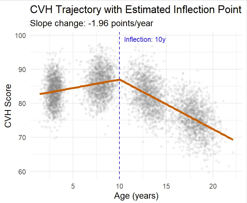
plot_model_fit <- function(original_data, model_list, best_psi) {
# 创建用于绘图的平滑数据网格
pred_grid <- expand.grid(
age = seq(min(original_data$age), max(original_data$age), length.out = 100),
exposure = unique(original_data$exposure), # 如果模型包含暴露因素
id = original_data$id[1] # 占位符,用于predict
)
# 如果是简单模型(未包含exposure交互),我们需要手动构造分段线
# 这里以 Grid Search 结果为例进行通用绘制
# 提取系数
coefs <- fixef(model_list$model)
b0 <- coefs["(Intercept)"]
b1 <- coefs["age"]
b2 <- coefs["age_spline_final"]
# 计算群体平均预测值
pred_grid$pred <- b0 + b1 * pred_grid$age +
b2 * pmax(0, pred_grid$age - best_psi)
p <- ggplot() +
# 1. 原始数据点 (背景)
geom_point(data = original_data, aes(x = age, y = cvh_score),
alpha = 0.1, color = "grey50") +
# 2. 模型拟合线 (加粗红色)
geom_line(data = pred_grid, aes(x = age, y = pred),
color = "#D55E00", linewidth = 1.5) +
# 3. 拐点垂直线
geom_vline(xintercept = best_psi, linetype = "dashed", color = "blue") +
# 4. 标注
annotate("text", x = best_psi + 0.5, y = max(original_data$cvh_score),
label = paste0("Inflection: ", round(best_psi, 1), "y"),
hjust = 0, color = "blue") +
labs(title = "CVH Trajectory with Estimated Inflection Point",
subtitle = paste("Slope change:", round(b2, 2), "points/year"),
y = "CVH Score", x = "Age (years)") +
theme_minimal(base_size = 14)
return(p)
}
# 绘制图形
p_final <- plot_model_fit(df, model_grid, model_grid$psi)
print(p_final)
# ============================================
# 6. 按暴露因素分层分析 (dplyr 管道化)
# ============================================
group_analysis <- df %>%
group_by(exposure) %>%
group_modify(~ {
# 对每组运行 grid search
res <- fit_grid_search_lme(.x, psi_seq = seq(8, 12, 0.5)) # 降低精度以加快演示速度
# 提取参数
extract_results(res$model, res$psi, "Subgroup Analysis")
}) %>%
ungroup()
print("=== 分层分析结果 ===")
print(group_analysis)

