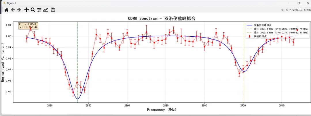
附上Python代码
import jsonimport numpy as npimport matplotlib.pyplot as pltfrom scipy.optimize import curve_fit# 读取JSON文件#with open('ODMR Spectrum_2025-11-12-14-47-17_FW_4P2K.txt', 'r', encoding='utf-8') as file:with open('ODMR Spectrum_2025-11-12-14-58-52_FW_4P4K.txt', 'r', encoding='utf-8') as file: data = json.load(file)# 提取实验数据点(带误差)experiment_data = Nonefor series in data['option']['series']: if series.get('name') == 'PL (a.u.)' and series.get('type') == 'custom': experiment_data = series break# 提取频率和强度数据frequencies = np.array([point[0] for point in experiment_data['data']])intensities = np.array([point[1] for point in experiment_data['data']])errors = np.array([point[2] for point in experiment_data['data']])# 定义洛伦兹函数模型(2个峰)def lorentzian_2peaks(x, *params): """ 2个洛伦兹峰叠加的函数 参数顺序: [offset, freq1, fwhm1, contrast1, freq2, fwhm2, contrast2] """ y = params[0] # offset for i in range(2): freq = params[1 + i * 3] fwhm = params[2 + i * 3] contrast = params[3 + i * 3] y += contrast * (fwhm / 2) ** 2 / ((x - freq) ** 2 + (fwhm / 2) ** 2) return y# 初始参数猜测(基于数据观察)# 选择两个最明显的峰(2835和2913 MHz附近)initial_guess = [ 1.0, # offset 2835, 6, -0.05, # 峰1: 频率, 半高宽, 对比度 2913, 6, -0.03 # 峰2]# 参数边界lower_bounds = [0.9] + [2800, 1, -0.1] * 2upper_bounds = [1.1] + [2950, 15, -0.01] * 2# 进行拟合try: popt, pcov = curve_fit( lorentzian_2peaks, frequencies, intensities, p0=initial_guess, sigma=errors, bounds=(lower_bounds, upper_bounds), maxfev=5000 ) # 计算拟合优度 fitted_intensities = lorentzian_2peaks(frequencies, *popt) residuals = intensities - fitted_intensities chisq = np.sum((residuals / errors) ** 2) r_squared = 1 - np.var(residuals) / np.var(intensities) print("双峰拟合成功!") print(f"R² = {r_squared:.6f}") print(f"χ² = {chisq:.6f}")except Exception as e: print(f"双峰拟合失败: {e}") # 使用简化的参数作为备选 popt = [1.0, 2835, 6, -0.05, 2913, 6, -0.03] print("使用默认参数")# 生成拟合曲线的高密度点fine_frequencies = np.linspace(frequencies.min(), frequencies.max(), 1000)fitted_curve = lorentzian_2peaks(fine_frequencies, *popt)# 提取拟合参数offset = popt[0]fit_params = []for i in range(2): freq = popt[1 + i * 3] fwhm = popt[2 + i * 3] contrast = popt[3 + i * 3] fit_params.append((freq, fwhm, contrast))# 设置中文字体plt.rcParams['font.sans-serif'] = ['Noto Sans CJK JP', 'SimHei', 'Arial']plt.rcParams['axes.unicode_minus'] = False# 创建图表plt.figure(figsize=(20, 5))# 绘制实验数据点(带误差棒)plt.errorbar(frequencies, intensities, yerr=errors, fmt='ro', markersize=4, capsize=3, capthick=1, elinewidth=1, label='实验数据点', zorder=5)# 用红线连接实验数据点plt.plot(frequencies, intensities, 'r-', linewidth=1, alpha=0.7, zorder=4)# 绘制拟合曲线plt.plot(fine_frequencies, fitted_curve, 'b-', linewidth=1.5, label='双洛伦兹峰拟合')# 添加拟合峰的位置标记colors = ['green', 'orange']for i, (freq, fwhm, contrast) in enumerate(fit_params): color = colors[i % len(colors)] label = f'峰{i + 1}: {freq:.1f} MHz (C={contrast:.4f}, FWHM={fwhm:.2f} MHz)' plt.axvline(x=freq, color=color, linestyle='--', alpha=0.7, linewidth=1, label=label)# 设置图表属性plt.title('ODMR Spectrum - 双洛伦兹峰拟合', fontsize=16)plt.xlabel('Frequency (MHz)', fontsize=14)plt.ylabel('Normalized PL (a.u.)', fontsize=14)plt.legend(fontsize=9, loc='upper right')plt.grid(True, alpha=0.3)# 添加拟合质量信息文本框fit_info = f'R² = {r_squared:.4f}\nχ² = {chisq:.2f}'plt.annotate(fit_info, xy=(0.02, 0.98), xycoords='axes fraction', fontsize=10, verticalalignment='top', bbox=dict(boxstyle='round', facecolor='wheat', alpha=0.8))# 调整布局并保存图表plt.tight_layout()plot_filename = "odmr_2peak_fit_with_red_line.png"plt.savefig(plot_filename, dpi=300, bbox_inches='tight')plt.show()print(f"双峰拟合的ODMR谱图已保存到 {plot_filename}")# 打印拟合参数详情print("\n双峰拟合参数详情:")print(f"基线 (offset): {offset:.6f}")for i, (freq, fwhm, contrast) in enumerate(fit_params): print(f"峰{i + 1}:") print(f" 共振频率: {freq:.2f} MHz") print(f" 半高全宽: {fwhm:.2f} MHz") print(f" 对比度: {contrast:.6f}")# 计算两个峰的频率差(可用于估算磁场)if len(fit_params) == 2: freq_diff = abs(fit_params[1][0] - fit_params[0][0]) print(f"\n两个峰的频率差: {freq_diff:.2f} MHz") # 对于NV色心,频率差与磁场的关系:Δf = γ * B,其中γ ≈ 2.8 MHz/mT # 磁场估算:B = Δf / γ gamma = 2.8 # MHz/mT magnetic_field = freq_diff / gamma print(f"估算磁场强度: {magnetic_field:.2f} mT")