顶刊中的全球地图投影（一）-常用投影

顶刊中的全球地图投影（二）-特殊投影

之前的文章介绍了一些地图投影以及如何基本的用途。这篇文章介绍怎么在代码中实现，并添加一些矢量与栅格数据进行绘图。

完整代码及数据均开源，获取方式见文末。

数据来源

接下来介绍一下待会会用到的数据，仅是用作演示，所以随便找了一些。数据的详细来源与处理方法见文末。点数据有两份，一份为陆地样点分布，一份为海洋样点分布；面数据为大洲边界数据；栅格数据为陆地DEM数据和全球DEM数据。

投影实现

投影对比

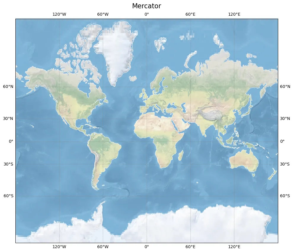
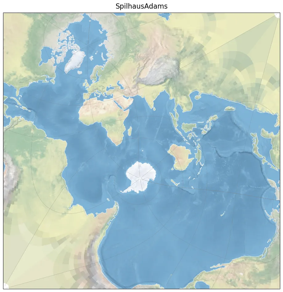
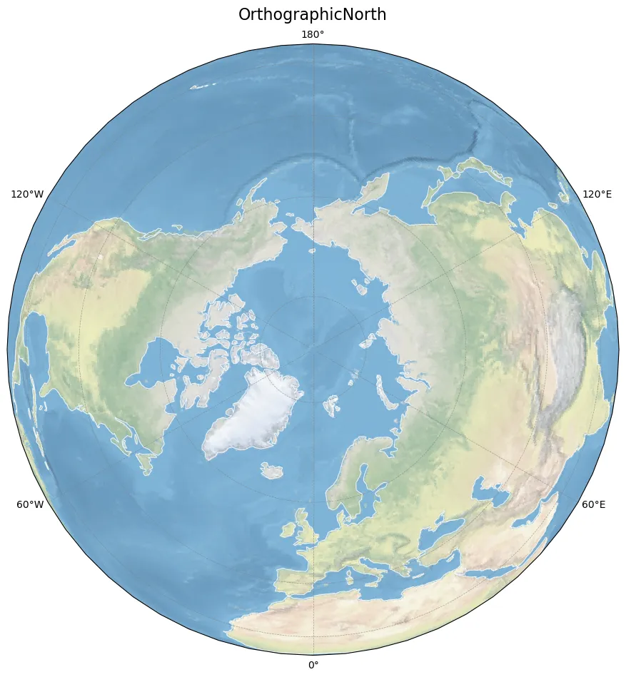
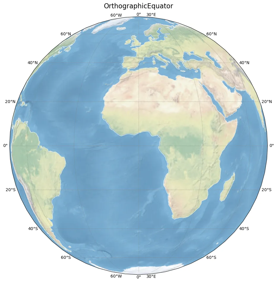
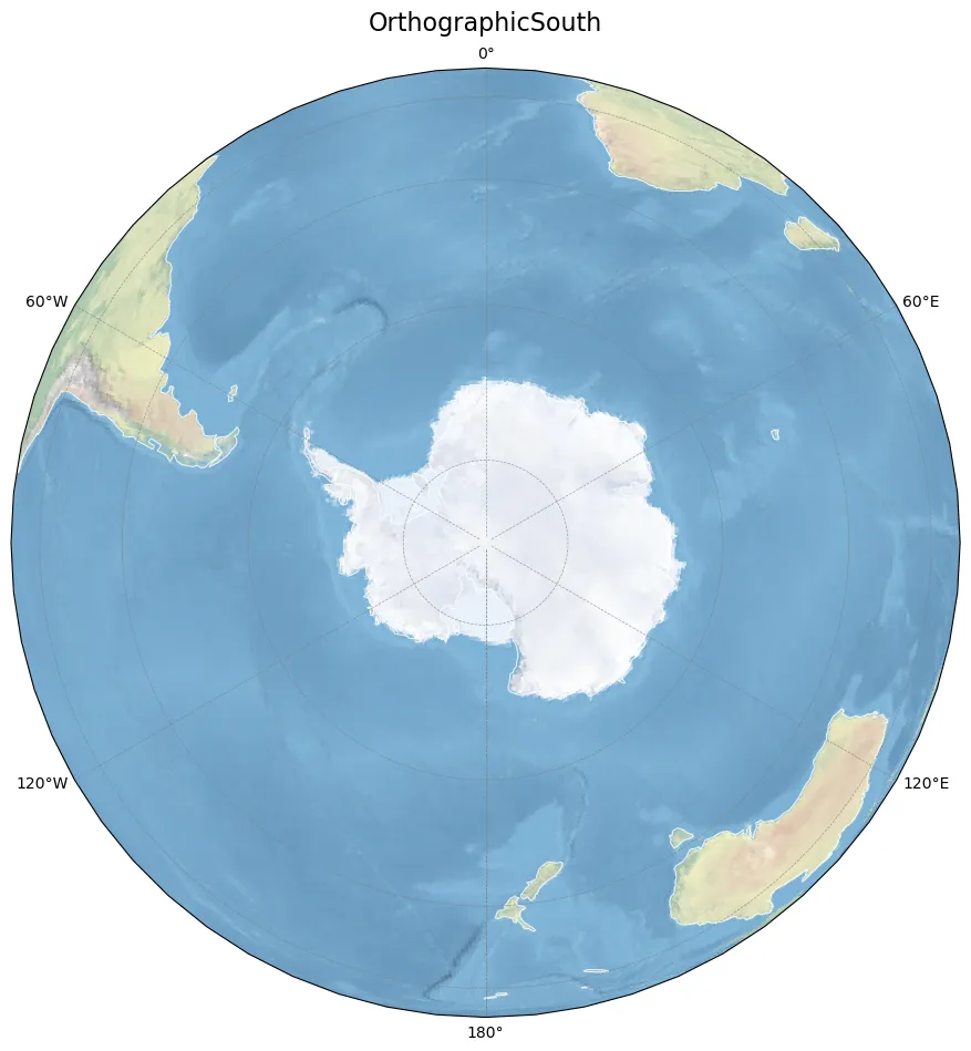
先用cartopy的默认底图，生成一些简单的地图，对比一下看看效果。

其中Spilhaus投影绘制的时间较长，大致为2分钟。

Spilhaus和Orthographic投影以下仅是最简单版本，实际使用会再调整，之后会再单独写一篇。

projections.py

"""-------------------------------------------------------------------------------@Author         :  zbhgis@Github         :  https://github.com/zbhgis@Description    :  generate some map-projection plots-------------------------------------------------------------------------------"""import matplotlib.pyplot as pltimport cartopy.crs as ccrsimport cartopy.feature as cfeatureimport time# 计时start_time = time.perf_counter()# 设置投影名称与对应的投影projections = [    ("Mercator", ccrs.Mercator()),    ("Robinson", ccrs.Robinson()),    ("EqualEarth", ccrs.EqualEarth()),    ("GoodeHomolosine", ccrs.InterruptedGoodeHomolosine()),    ("SpilhausAdams", ccrs.Spilhaus()),    ("OrthographicNorth", ccrs.Orthographic(central_longitude=0, central_latitude=90)),    ("OrthographicEquator", ccrs.Orthographic(central_longitude=0, central_latitude=0)),    ("OrthographicSouth", ccrs.Orthographic(central_longitude=0, central_latitude=-90)),]# 每个投影一张图片for proj_name, proj in projections:    fig = plt.figure(figsize=(10, 10))    ax = fig.add_subplot(1, 1, 1, projection=proj)    ax.set_global()    ax.stock_img()    ax.add_feature(        cfeature.COASTLINE,        linewidth=0.8,        edgecolor="white",        alpha=0.8,    )    ax.gridlines(        draw_labels=True,        linewidth=0.5,        color="gray",        linestyle="--",        alpha=0.7,    )    ax.set_title(proj_name, fontsize=16, pad=10)    print(proj_name)    plt.tight_layout(rect=[0, 0, 1, 0.96])    plt.savefig(f"./fig_res/world_maps_{proj_name}.png", dpi=100, bbox_inches="tight")    plt.close(fig)end_time = time.perf_counter()print(end_time - start_time)

打印结果

MercatorRobinsonEqualEarthGoodeHomolosineSpilhausAdamsOrthographicNorthOrthographicEquatorOrthographicSouth159.37829679995775

绘制结果

Mercator

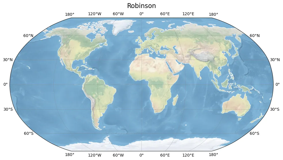
Robinson

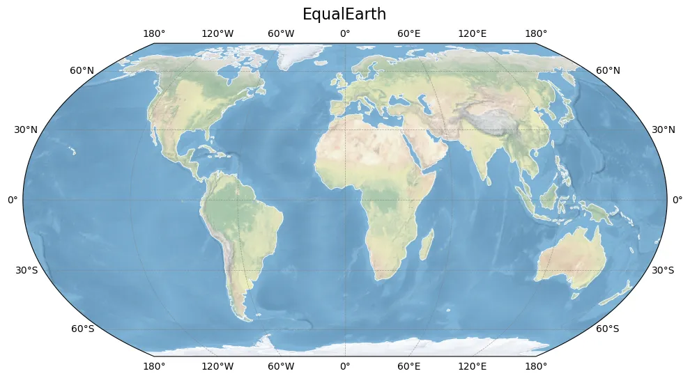
EqualEarth

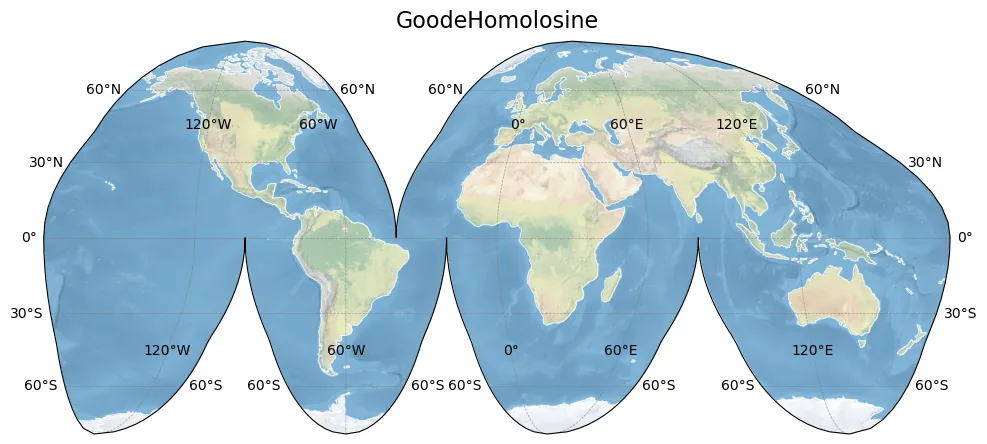
Goode

Spilhaus

OrthographicNorth

OrthographicEquator

OrthographicSouth

添加数据

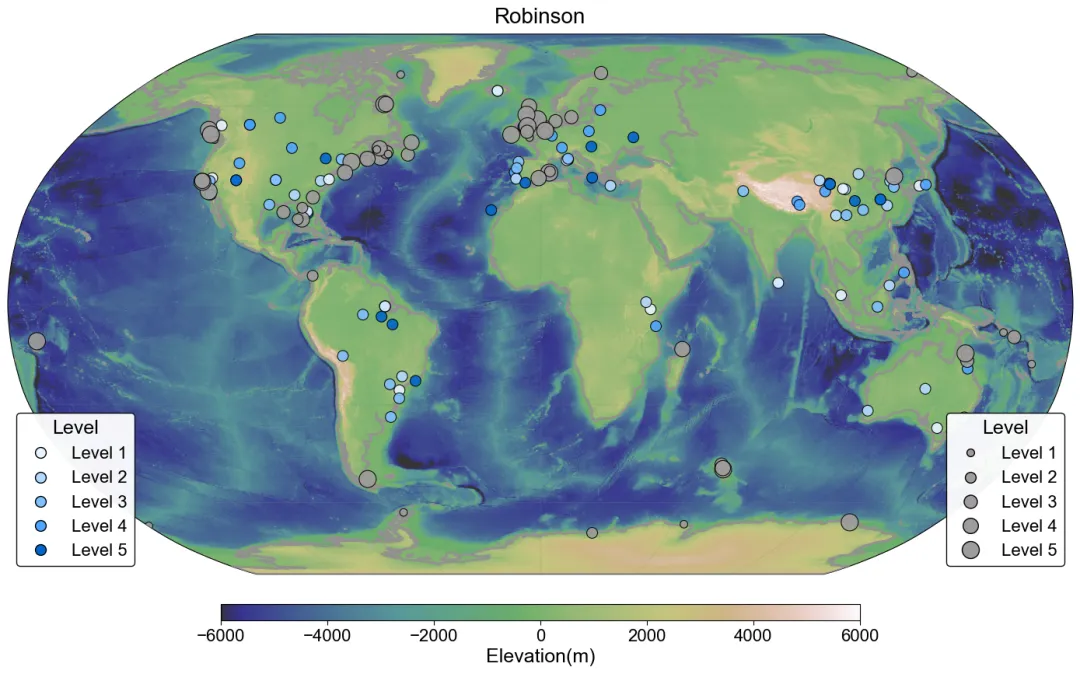
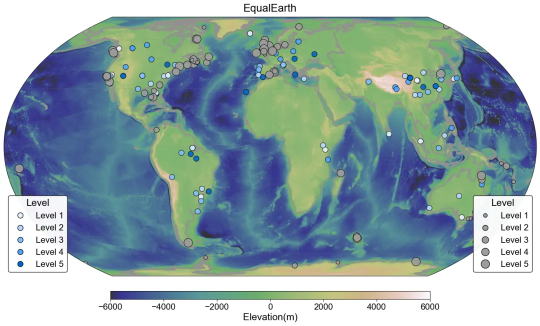
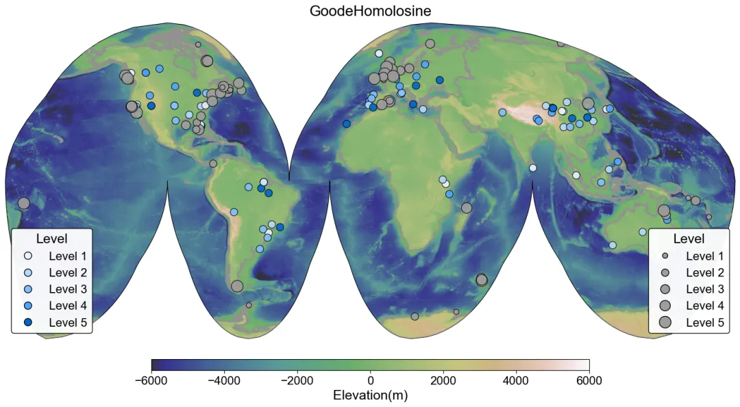
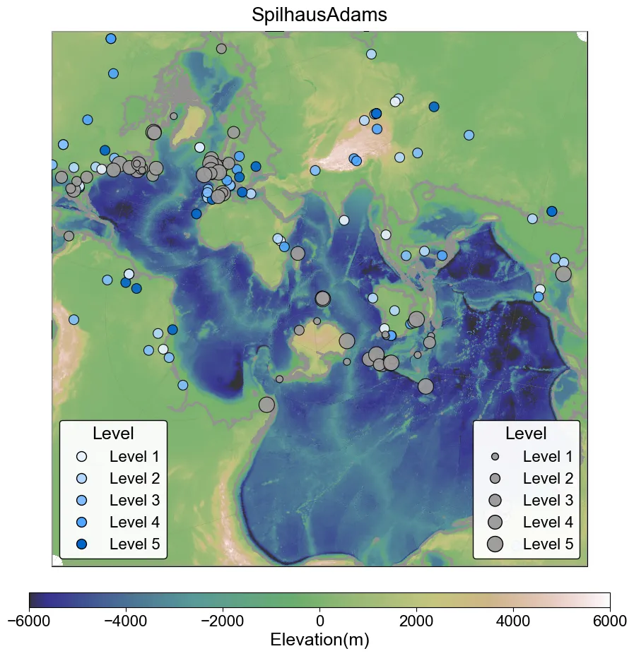
在上述代码的基础上，进一步添加数据进行制图。先通过rasterio包添加全球DEM数据与色带，然后再添加边界数据，最后分别添加样点数据（样点数据分布与对应值无实际含义，仅供演示）。

代码没啥难度，主要调整细节麻烦了一点，以下代码没有考虑科研风格，只是简单绘制了一下，之后会单独出一个系列来复现科研地图的。

以下是整理好的Python脚本，文末也提供了Jupyter Notebook格式的脚本，方便理解绘图过程与思路。

这行代码调整id即可绘制出对应的投影，大家根据需要调整即可，默认为Robinson投影。

proj_name, proj_obj = projections[1]

plot.py

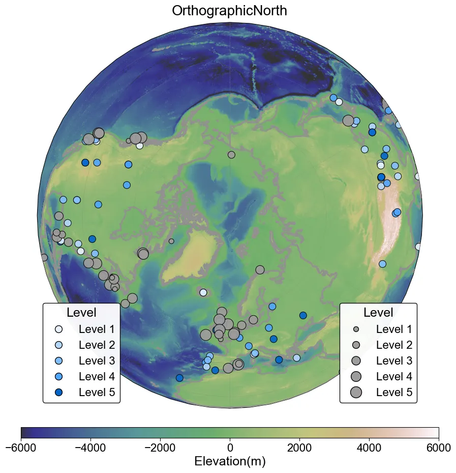
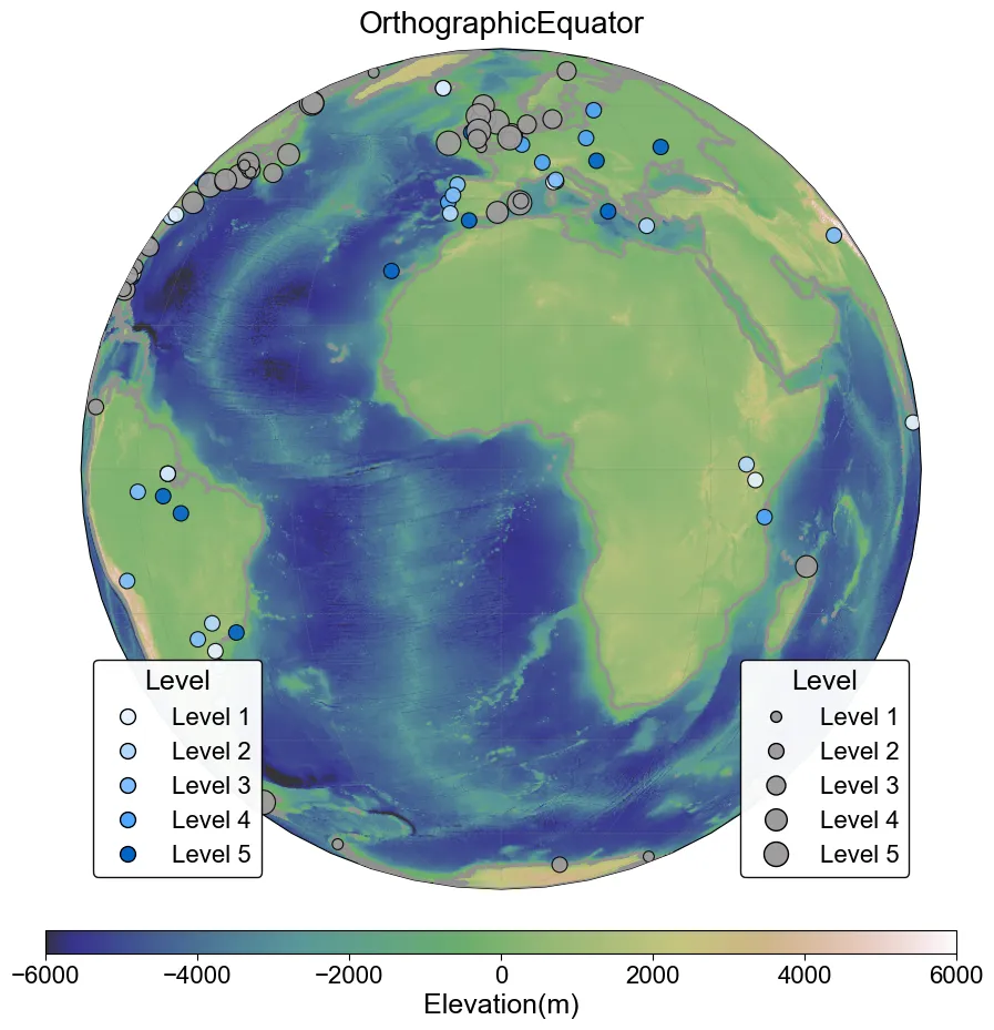
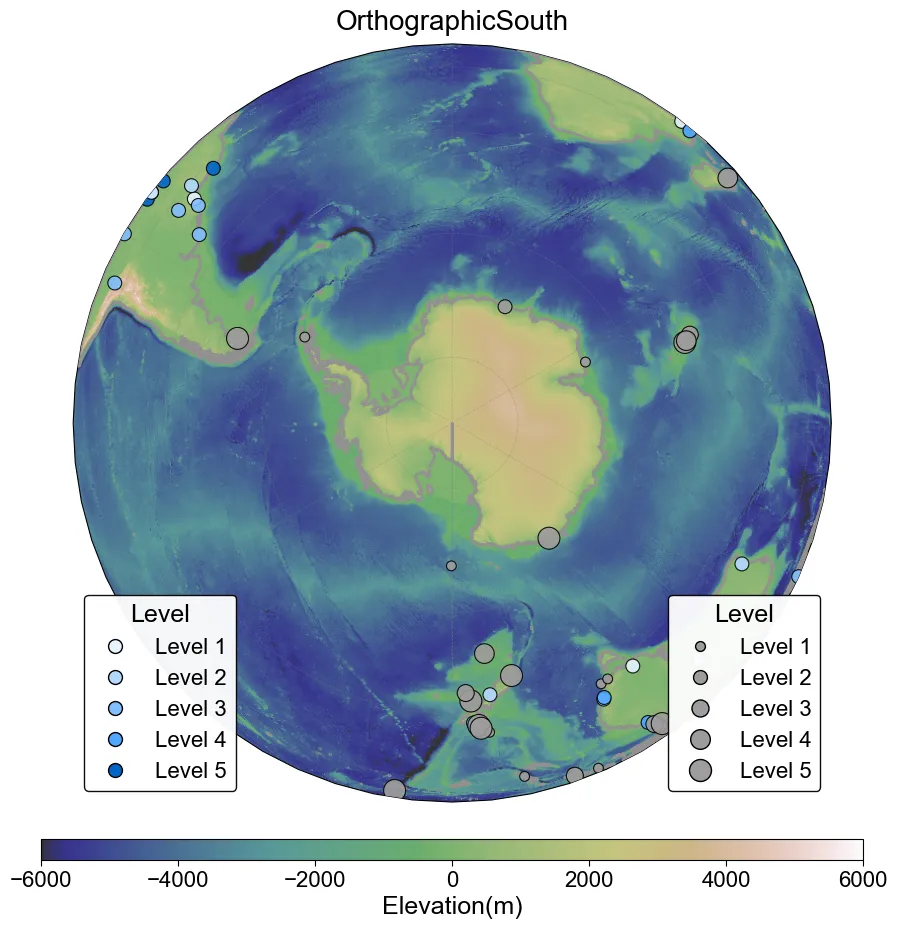
"""-------------------------------------------------------------------------------@Author         :  zbhgis@Github         :  https://github.com/zbhgis@Description    :  add some vector and raster data on map-projection plots-------------------------------------------------------------------------------"""import matplotlib.pyplot as pltimport cartopy.crs as ccrsimport cartopy.feature as cfeatureimport cartopy.io.shapereader as shpreaderimport rasterioimport geopandas as gpdfrom matplotlib.lines import Line2Dimport numpy as npplt.rcParams["font.family"] = "Arial"boundary_shp = "./data_res/boundary.shp"points_land_shp = "./data_res/points_land.shp"points_ocean_shp = "./data_res/points_ocean.shp"dem_tif = "./data_res/gebco_dem.tif"fig = plt.figure(figsize=(14, 10), dpi=100)projections = [    ("Mercator", ccrs.Mercator()),    ("Robinson", ccrs.Robinson()),    ("EqualEarth", ccrs.EqualEarth()),    ("GoodeHomolosine", ccrs.InterruptedGoodeHomolosine()),    ("SpilhausAdams", ccrs.Spilhaus()),    ("OrthographicNorth", ccrs.Orthographic(central_longitude=0, central_latitude=90)),    ("OrthographicEquator", ccrs.Orthographic(central_longitude=0, central_latitude=0)),    ("OrthographicSouth", ccrs.Orthographic(central_longitude=0, central_latitude=-90)),]proj_name, proj_obj = projections[1]ax = fig.add_subplot(1, 1, 1, projection=proj_obj)ax.set_global()# 添加DEM数据with rasterio.open(dem_tif) as src:    dem_data = src.read(1, masked=True)    left, bottom, right, top = src.bounds    extent = [left, right, bottom, top]    im = ax.imshow(        dem_data,        extent=extent,        transform=ccrs.PlateCarree(),        origin="upper",        cmap="gist_earth",        vmin=-6000,        vmax=6000,        alpha=0.8,        interpolation="bilinear",    )# 添加DEM色带cbar = fig.colorbar(    im,    ax=ax,    orientation="horizontal",    pad=0.04,    aspect=40,    shrink=0.6,)cbar.ax.tick_params(    labelsize=16,    labelcolor="black",    length=4,)cbar.set_label("Elevation(m)", fontsize=18)# 添加矢量边界数据reader = shpreader.Reader(boundary_shp)boundary_feature = cfeature.ShapelyFeature(    reader.geometries(),    ccrs.PlateCarree(),    facecolor="none",    edgecolor="#928F8F",    linewidth=2.0,    linestyle="-",)ax.add_feature(boundary_feature, zorder=10)# 添加陆地点数据gdf = gpd.read_file(points_land_shp)lons = gdf.geometry.xlats = gdf.geometry.y# 生成陆地点数据颜色color_map_land = {1: "#E6F3FF",2: "#B3D9FF",3: "#80BFFF",4: "#4DA6FF",5: "#0066CC",}colors = [color_map_land.get(level, "gray") for level in gdf["level"]]# 绘制陆地点数据ax.scatter(    lons,    lats,    s=100,    c=colors,    edgecolor="black",    linewidth=0.8,    alpha=0.9,    transform=ccrs.PlateCarree(),    zorder=10,)# 添加陆地点图例legend_elements_land = [    Line2D(        [0],        [0],        marker="o",        linestyle="none",        label=f"Level {l}",        markerfacecolor=color,        markersize=10,        markeredgecolor="black",    )for l, color in color_map_land.items()]legend_land = ax.legend(    handles=legend_elements_land,    loc="lower left",    title="Level",    title_fontsize=18,    fontsize=16,    frameon=True,    edgecolor="black",    facecolor="white",    framealpha=0.95,)legend_land.set_zorder(15)ax.add_artist(legend_land)# 相同方法再添加一次海洋点数据gdf = gpd.read_file(points_ocean_shp)lons = gdf.geometry.xlats = gdf.geometry.y# 生成海洋点数据尺寸size_map_ocean = {1: 50,2: 100,3: 150,4: 200,5: 250,}sizes = [size_map_ocean.get(level, 0) for level in gdf["level"]]# 绘制海洋点数据ax.scatter(    lons,    lats,    s=sizes,    c="#9F9C9C",    edgecolor="black",    linewidth=0.8,    alpha=0.9,    transform=ccrs.PlateCarree(),    zorder=10,)# 添加海洋点图例legend_elements_ocean = [    Line2D(        [0],        [0],        marker="o",        linestyle="none",        label=f"Level {s}",        markerfacecolor="#9F9C9C",        markersize=np.sqrt(size),        markeredgecolor="black",    )for s, size in size_map_ocean.items()]legend_ocean = ax.legend(    handles=legend_elements_ocean,    loc="lower right",    title="Level",    title_fontsize=18,    fontsize=16,    frameon=True,    edgecolor="black",    facecolor="white",    framealpha=0.95,)legend_ocean.set_zorder(15)# 添加经纬度标签gl = ax.gridlines(    draw_labels=False,    linewidth=0.5,    color="gray",    alpha=0.4,    linestyle="--",)# 添加图名ax.set_title(proj_name, fontsize=20, pad=10)plt.tight_layout()plt.savefig(f"./fig_res/gebco_dem_{proj_name}.png",    dpi=100,    bbox_inches="tight",    facecolor="white",)print("ok")

打印结果

ok

绘制结果

Mercator

Robinson

EqualEarth

GoodeHomolosine

Spilhaus

OrthographicNorth

OrthographicEquator

OrthographicSouth

数据处理方法

接下来是数据的来源以及详细的处理方法，感兴趣的了解一下即可。

点数据

点数据来自于以下的2篇生物多样性文献：

Keck, F., Peller, T., Alther, R. et al. The global human impact on biodiversity. Nature 641, 395–400 (2025). https://doi.org/10.1038/s41586-025-08752-2Carter, H.F., Bribiesca-Contreras, G. & Williams, S.T. Deep-sea-floor diversity in Asteroidea is shaped by competing processes across different latitudes and oceans. Nat Ecol Evol 9, 1910–1923 (2025). https://doi.org/10.1038/s41559-025-02808-2

在以下网址中中提供了所有数据：

https://github.com/fkeck/metabeta/tree/main

https://data.nhm.ac.uk/dataset/global-asteroidea-occurrence-data

下载文献的data.json和Global Asteroidea Occurrence Dataset.json后，通过以下Python代码将分别将数据简化为100条，并转为shp格式，保留坐标字段，并新建一个随机等级字段（用于配色）。

json2shp.py

"""-------------------------------------------------------------------------------@Author         :  zbhgis@Github         :  https://github.com/zbhgis@Description    :  convert json to shapefile-------------------------------------------------------------------------------"""import jsonimport randomimport pandas as pdimport geopandas as gpdfrom shapely.geometry import Pointdefjson2shp(    json_path,    output_shp_path,    keep_count=100,    lon_field="Longitude",    lat_field="Latitude",    crs="EPSG:4326",):# 打开数据with open(json_path, "r", encoding="utf-8") as f:        data = json.load(f)# 数据抽样    sampled_data = random.sample(data, keep_count)    df = pd.DataFrame(sampled_data)    df = df[[lon_field, lat_field]]# 字段重命名    df = df.rename(columns={lon_field: "lon", lat_field: "lat"})    df["lon"] = pd.to_numeric(df["lon"], errors="coerce")    df["lat"] = pd.to_numeric(df["lat"], errors="coerce")# 颜色字段    df["level"] = [random.randint(1, 5) for _ in range(len(df))]# 生成gdf    geometry = [Point(xy) for xy in zip(df["lon"], df["lat"])]    gdf = gpd.GeoDataFrame(        df.drop(columns=["lon", "lat"]),        geometry=geometry,        crs=crs,    )    gdf.to_file(output_shp_path, encoding="utf-8")if __name__ == "__main__":    json_file = "./data_origin/data.json"    shp_file = "./data_res/points_land.shp"    json2shp(        json_path=json_file,        output_shp_path=shp_file,        keep_count=100,        lon_field="Longitude",        lat_field="Latitude",        crs="EPSG:4326",    )    json_file = "./data_origin/resource.json"    shp_file = "./data_res/points_ocean.shp"    json2shp(        json_path=json_file,        output_shp_path=shp_file,        keep_count=100,        lon_field="Long",        lat_field="Lat",        crs="EPSG:4326",    )    print("OK")

打印结果

OK

面数据

面数据是一份很早之前在网上下载的大洲边界矢量数据，通过以下Python代码检查一下数据。

check_shp.py

"""-------------------------------------------------------------------------------@Author         :  zbhgis@Github         :  https://github.com/zbhgis@Description    :  check and copy shapefile-------------------------------------------------------------------------------"""import geopandas as gpdimport osimport shutildefcheck_file(shp_path):    gdf = gpd.read_file(shp_path)if gdf.crs isNone:        print("未定义坐标系")elif gdf.crs.to_epsg() == 4326:        print("EPSG:4326")elif gdf.crs.to_epsg() isnotNone:        print(f"EPSG:{gdf.crs.to_epsg()}")defcopy_shapefile(shp_path, output_folder, new_base_name):    base_dir = os.path.dirname(shp_path)    base_name = os.path.splitext(os.path.basename(shp_path))[0]    extensions = [".shp", ".shx", ".dbf", ".prj", ".cpg", ".sbn", ".sbx", ".shp.xml"]    copied = 0for ext in extensions:        src_file = os.path.join(base_dir, base_name + ext)if os.path.exists(src_file):            dst_file = os.path.join(output_folder, new_base_name + ext)            shutil.copy2(src_file, dst_file)            copied += 1if copied > 0:        print(f"成功复制")else:        print("复制失败")if __name__ == "__main__":    shp = "./data_origin/continent.shp"    target_folder = "./data_res"    check_file(shp)    copy_shapefile(shp, target_folder, "boundary")

打印结果

EPSG:4326成功复制

栅格数据

栅格数据是通过GEE下载的DEM数据，通过以下js代码重采样为10km分辨率并下载至本地。

陆地DEM下载

数据介绍：https://developers.google.com/earth-engine/datasets/catalog/COPERNICUS_DEM_GLO30

cop_download.js

var dataset = ee.ImageCollection("COPERNICUS/DEM/GLO30");var elevation = dataset.select("DEM").mosaic();var elevationVis = {min: 0.0,max: 1000.0,palette: ["0000ff", "00ffff", "ffff00", "ff0000", "ffffff"],};Map.setCenter(-6.746, 46.529, 4);Map.addLayer(elevation, elevationVis, "DEM");Export.image.toDrive({crs: "EPSG:4326",image: elevation,description: "WORLD_Elevation",scale: 10000,maxPixels: 1e13,});

全球DEM下载

数据介绍：https://gee-community-catalog.org/projects/gebco/

gebco_download.js

var dataset = ee.ImageCollection("projects/sat-io/open-datasets/gebco/gebco_grid",);var elevation = dataset.select("b1").mosaic();var elevationVis = {min: -7000.0,max: 5000.0,palette: ["0000ff", "00ffff", "ffff00", "ff0000", "ffffff"],};Map.setCenter(-37.62, 25.8, 2);Map.addLayer(elevation, elevationVis, "b1");Export.image.toDrive({crs: "EPSG:4326",image: elevation,description: "GEBCO_Elevation",scale: 10000,maxPixels: 1e13,});

写在最后

完整代码及相关数据文件会在以下github仓库中开源，若有帮助欢迎点个star，不胜感激。

https://github.com/zbhgis/Projects

或者在微信公众号后台回复关键词“代码获取”即可获取百度网盘链接，找到对应名称的文件夹即可（百度网盘链接可能隔几天才会同步）。

代码中使用了很多相对路径，建议获取的时候下载完整文件夹。

该系列下一篇会再对Spilhaus和Orthographic投影绘制进行补充。

如有问题，欢迎添加个人微信交流。