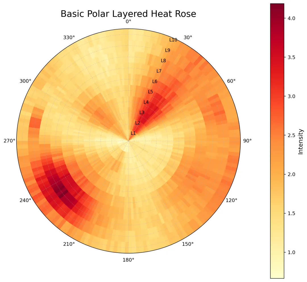
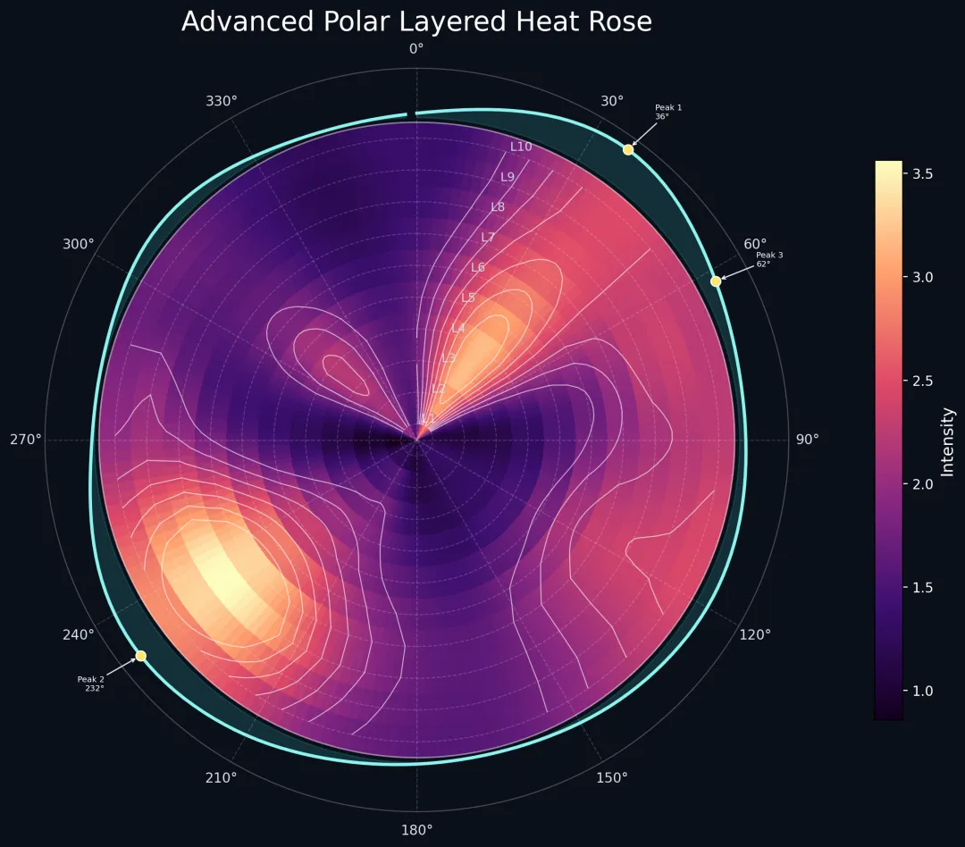
import osimport numpy as npimport matplotlib.pyplot as pltfrom matplotlib.colors import LinearSegmentedColormap# 0. 输出目录OUTDIR = "polar_rose_output"os.makedirs(OUTDIR, exist_ok=True)# 1. 构造模拟数据def ang_diff_deg(a, b): """计算角度差(单位:度),结果限制在 [-180, 180]""" return (a - b + 180) % 360 - 180def gaussian_ang(theta_deg, mu_deg, sigma_deg): d = ang_diff_deg(theta_deg, mu_deg) return np.exp(-0.5 * (d / sigma_deg) ** 2)def generate_polar_layer_data(n_theta=180, n_r=10, seed=2026): """ 构造“方向-层级-强度”三维数据 theta: 方向 r: 层级 Z: 每个方向-层级组合对应的强度 """ rng = np.random.default_rng(seed) theta_centers = np.linspace(0, 360, n_theta, endpoint=False) # degree r_centers = np.arange(1, n_r + 1) T, R = np.meshgrid(theta_centers, r_centers) # 多个方向主峰 peak1 = 1.8 * gaussian_ang(T, 35, 18) * (0.65 + 0.35 * np.exp(-((R - 3.0) / 2.2) ** 2)) peak2 = 1.5 * gaussian_ang(T, 120, 26) * (0.45 + 0.55 * np.exp(-((R - 6.5) / 1.8) ** 2)) peak3 = 1.9 * gaussian_ang(T, 235, 20) * (0.35 + 0.75 * np.exp(-((R - 8.0) / 1.5) ** 2)) peak4 = 1.2 * gaussian_ang(T, 310, 15) * (0.60 + 0.40 * np.exp(-((R - 4.0) / 1.7) ** 2)) # 条带型起伏 band = 0.35 * (1 + np.cos(np.deg2rad(2.2 * T - 18 * R))) wave = 0.25 * (1 + np.sin(np.deg2rad(1.3 * T + 25 * R))) # 径向趋势 radial_trend = 0.15 + 0.08 * R + 0.12 * np.exp(-((R - 5.5) / 3.2) ** 2) # 局部热点 hotspot = ( 0.9 * gaussian_ang(T, 70, 8) * np.exp(-((R - 8.5) / 0.9) ** 2) + 0.8 * gaussian_ang(T, 205, 10) * np.exp(-((R - 2.5) / 0.8) ** 2) + 1.1 * gaussian_ang(T, 280, 7) * np.exp(-((R - 9.0) / 0.7) ** 2) ) noise = 0.08 * rng.normal(size=(n_r, n_theta)) Z = peak1 + peak2 + peak3 + peak4 + band + wave + radial_trend + hotspot + noise Z = np.clip(Z, 0, None) return theta_centers, r_centers, Z# 2. 平滑函数def circular_smooth_along_theta(Z, kernel_size=11, sigma=2.8): """ 对角度方向做环形平滑 Z shape = (n_r, n_theta) """ x = np.arange(kernel_size) - kernel_size // 2 kernel = np.exp(-0.5 * (x / sigma) ** 2) kernel /= kernel.sum() pad = kernel_size // 2 Z_pad = np.concatenate([Z[:, -pad:], Z, Z[:, :pad]], axis=1) out = np.zeros_like(Z) for i in range(Z.shape[0]): out[i] = np.convolve(Z_pad[i], kernel, mode="valid") return outdef smooth_along_radius(Z, kernel_size=5, sigma=1.1): """ 对径向做一维平滑 """ x = np.arange(kernel_size) - kernel_size // 2 kernel = np.exp(-0.5 * (x / sigma) ** 2) kernel /= kernel.sum() pad = kernel_size // 2 Z_pad = np.pad(Z, ((pad, pad), (0, 0)), mode="edge") out = np.zeros_like(Z) for j in range(Z.shape[1]): out[:, j] = np.convolve(Z_pad[:, j], kernel, mode="valid") return out# 3. 找主方向峰值def find_top_direction_peaks(theta_deg, profile, min_sep_deg=22, top_k=3): """ 在方向强度曲线上找几个主峰,避免彼此过近 """ idx_sorted = np.argsort(profile)[::-1] chosen = [] for idx in idx_sorted: ang = theta_deg[idx] good = True for c in chosen: if abs(ang_diff_deg(ang, theta_deg[c])) < min_sep_deg: good = False break if good: chosen.append(idx) if len(chosen) >= top_k: break return chosen# 4. 作图:基础版def plot_basic(theta_deg, r_centers, Z, out_png): fig = plt.figure(figsize=(9, 9), dpi=220) ax = plt.subplot(111, projection="polar") # 构造边界 theta_edges = np.linspace(0, 2 * np.pi, len(theta_deg) + 1) r_edges = np.arange(0.5, len(r_centers) + 1.5, 1.0) mesh = ax.pcolormesh( theta_edges, r_edges, Z, cmap="YlOrRd", shading="auto" ) ax.set_theta_zero_location("N") ax.set_theta_direction(-1) ax.set_rlim(0.5, len(r_centers) + 0.5) ax.set_thetagrids( np.arange(0, 360, 30), labels=[f"{d}°" for d in range(0, 360, 30)], fontsize=10 ) ax.set_rgrids( np.arange(1, len(r_centers) + 1), angle=22.5, labels=[f"L{i}" for i in range(1, len(r_centers) + 1)], fontsize=9 ) ax.grid(alpha=0.35, linestyle="--", linewidth=0.7) ax.set_title("Basic Polar Layered Heat Rose", fontsize=18, pad=24) cbar = plt.colorbar(mesh, ax=ax, pad=0.10, shrink=0.88) cbar.set_label("Intensity", fontsize=12) plt.tight_layout() plt.savefig(out_png, bbox_inches="tight", facecolor="white")# 5. 作图:进阶版def plot_advanced(theta_deg, r_centers, Z, out_png): # 平滑后的热力场 Zs = circular_smooth_along_theta(Z, kernel_size=13, sigma=3.0) Zs = smooth_along_radius(Zs, kernel_size=5, sigma=1.0) # 方向积分强度,用于外环曲线 dir_profile = Zs.sum(axis=0) # 角度转弧度 theta = np.deg2rad(theta_deg) theta_edges = np.linspace(0, 2 * np.pi, len(theta_deg) + 1) r_edges = np.arange(0.5, len(r_centers) + 1.5, 1.0) # 自定义漂亮一点的配色 colors = ["#14001f", "#3b0f70", "#8c2981", "#de4968", "#fe9f6d", "#fcfdbf"] cmap_adv = LinearSegmentedColormap.from_list("custom_rose", colors, N=256) fig = plt.figure(figsize=(10, 10), dpi=240, facecolor="#0b0f1a") ax = plt.subplot(111, projection="polar", facecolor="#0b0f1a") # 主热力图 mesh = ax.pcolormesh( theta_edges, r_edges, Zs, cmap=cmap_adv, shading="auto" ) # 叠加等值线 tt, rr = np.meshgrid(theta, r_centers) levels = np.linspace(np.percentile(Zs, 50), np.percentile(Zs, 96), 7) cs = ax.contour( tt, rr, Zs, levels=levels, colors="white", linewidths=0.75, alpha=0.62 ) # 外环方向强度曲线 prof_norm = (dir_profile - dir_profile.min()) / (dir_profile.max() - dir_profile.min() + 1e-12) outer_base = len(r_centers) + 0.65 outer_curve = outer_base + 1.15 * prof_norm ax.plot(theta, outer_curve, color="#8ef9f3", lw=2.4, alpha=0.98) ax.fill_between(theta, outer_base, outer_curve, color="#38d9d9", alpha=0.16) # 标出主方向峰值 peak_ids = find_top_direction_peaks(theta_deg, dir_profile, min_sep_deg=26, top_k=3) for i, idx in enumerate(peak_ids, 1): ang = theta[idx] rr_peak = outer_curve[idx] deg = theta_deg[idx] ax.scatter( [ang], [rr_peak], s=55, c="#ffe66d", edgecolors="white", linewidths=0.8, zorder=8 ) r_text = rr_peak + 1.45 if 0 <= deg < 90: ha = "left" elif 90 <= deg < 180: ha = "left" elif 180 <= deg < 270: ha = "right" else: ha = "right" ax.annotate( f"Peak {i}\n{deg:.0f}°", xy=(ang, rr_peak), xytext=(ang, r_text), color="white", fontsize=6, ha=ha, va="center", arrowprops=dict( arrowstyle="->", color="white", lw=0.9, alpha=0.9, shrinkA=0, shrinkB=4 ) ) th_dense = np.linspace(0, 2*np.pi, 500) ax.plot(th_dense, np.full_like(th_dense, len(r_centers) + 0.5), color="white", lw=1.1, alpha=0.45) ax.set_theta_zero_location("N") ax.set_theta_direction(-1) ax.set_rlim(0.5, len(r_centers) + 2.2) ax.set_thetagrids( np.arange(0, 360, 30), labels=[f"{d}°" for d in range(0, 360, 30)], fontsize=10, color="#d9e2ec" ) ax.set_rgrids( np.arange(1, len(r_centers) + 1), angle=18, labels=[f"L{i}" for i in range(1, len(r_centers) + 1)], fontsize=9, color="#cbd5e1" ) ax.grid(color="white", alpha=0.18, linestyle="--", linewidth=0.75) ax.spines["polar"].set_color((1, 1, 1, 0.25)) ax.set_title( "Advanced Polar Layered Heat Rose", fontsize=20, color="white", pad=28 ) cbar = plt.colorbar(mesh, ax=ax, pad=0.10, shrink=0.6,fraction=0.035 ) cbar.set_label("Intensity", fontsize=12, color="white") cbar.ax.yaxis.set_tick_params(color="white") plt.setp(cbar.ax.get_yticklabels(), color="white") plt.tight_layout() plt.savefig(out_png, bbox_inches="tight", facecolor=fig.get_facecolor())def main(): theta_deg, r_centers, Z = generate_polar_layer_data() basic_png = os.path.join(OUTDIR, "polar_rose_basic.png") adv_png = os.path.join(OUTDIR, "polar_rose_advanced.png") plot_basic(theta_deg, r_centers, Z, basic_png) plot_advanced(theta_deg, r_centers, Z, adv_png)if __name__ == "__main__": main()