前置阅读:图神经网络:原理、算法与分子建模入门(图、消息传递、PyG 字段);需要三维几何与对称性时再读 SE(3)-等变图神经网络。PDB 文件字段含义可对照 PDB 格式说明。
本文只谈数据层:如何把「一个蛋白结构文件」变成 GNN 能吃的 Data(x, edge_index, pos, …),并对途中每一类 Python 数据结构建立整体印象。
段末注释:PyTorch Geometric(PyG) 是 PyTorch 上的图深度学习扩展库;BioPython 是常用的生物序列/结构解析 Python 包;mmCIF 为 PDB 的现代化文本格式。
1. 端到端数据流(先建立地图)
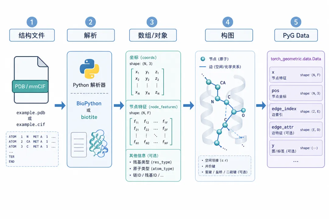 蛋白结构到 GNN:文件 → 解析 → 数组 → 图 → PyG Data
图 1(科普示意):实践中的主路径可概括为五步。
| | | |
|---|
| .pdb | | str |
| | | |
| | | numpy.ndarray |
| | | edge_index[2, E] |
| | | torch_geometric.data.Data |
结构编码在 GNN 语境下指:用图 把三维构象离散化,并把每个节点 编成特征向量 (可选边特征 、坐标 ),供消息传递学习 乃至图级 。
2. 结构文件里有什么
实验或预测结构常见 PDB(Protein Data Bank 文本格式)与 mmCIF(macromolecular Crystallographic Information File)。对 GNN 最重要的是:
- 谁:残基名、链 ID、残基序号、原子名(
CA = ) - 可选置信度:预测结构常把 pLDDT(predicted Local Distance Difference Test)写在 B-factor 列
一条 ATOM 行(概念分区,列宽以 wwPDB 文档 为准)包含:原子坐标、占有率、温度因子 B 等。GNN 构图时通常不把整行原样喂进网络,而是抽取成数值张量。
3. Python 中的结构表示:三层结构
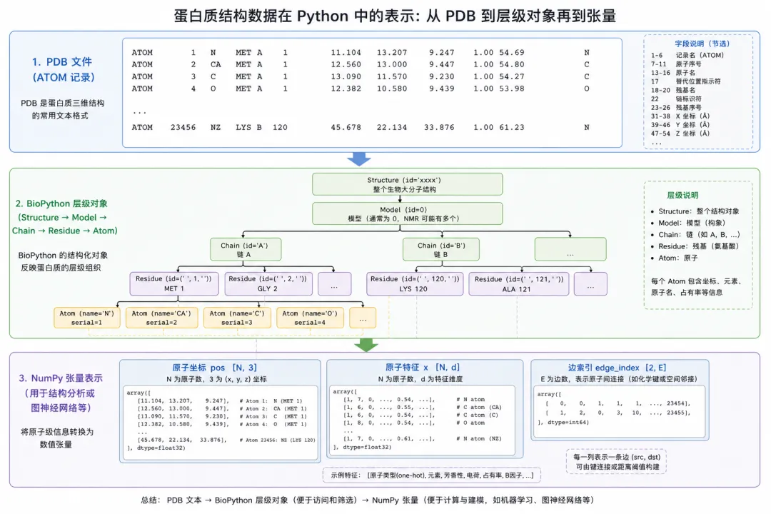 三层:文件行 → BioPython 对象树 → NumPy/PyTorch 张量
图 2(科普示意):同一份结构在内存里会同时存在「对象树」与「扁平张量」两种视图,后者才直接对接 GNN。
3.1 层次对象(BioPython)
BioPython 的 PDB 解析器(Bio.PDB.PDBParser)把文件读成:
Structure(id)          # 一个文件常对应一个 Structure(或 NMR 多模型)
 └── Model(id)
      └── Chain(id)
           └── Residue(resname, seqid, icode)
                └── Atom(name)
- 适合:按链筛选、跳过 HETATM、访问
residue.get_resname() 等语义操作
3.2 扁平张量(NumPy / PyTorch)
GNN 实际使用的是「表格式」数据:
| | |
|---|
pos | [N, 3] | |
x | [N, F] | 节点特征(氨基酸类型 one-hot、B-factor、pLDDT 等) |
edge_index | [2, E] | |
edge_attr | [E, D_e] | |
seq_pos | [N] | |
3.3 其它常用库(选型)
| | |
|---|
| BioPython | | |
| biotite | | |
| MDAnalysis | | |
| ASE | | |
下文示例以 BioPython + PyTorch + PyG 为主,换 biotite 时只需把「对象树 → pos/x」一步改成 AtomArray 索引。
4. 步骤 ①②:解析 PDB 并提取
from pathlib import Path
import numpy as np
import torch
from Bio.PDB import PDBParser

# 三字母氨基酸 -> 整数编号(可按项目扩展为 20+1 维 one-hot)
AA3_TO_IDX = {
"ALA": 0, "ARG": 1, "ASN": 2, "ASP": 3, "CYS": 4,
"GLN": 5, "GLU": 6, "GLY": 7, "HIS": 8, "ILE": 9,
"LEU": 10, "LYS": 11, "MET": 12, "PHE": 13, "PRO": 14,
"SER": 15, "THR": 16, "TRP": 17, "TYR": 18, "VAL": 19,
}

defextract_ca_table(pdb_path: str | Path, chain_id: str = "A", model_id: int = 0):
"""从一条链提取 Cα:坐标、氨基酸编号、B-factor(可作 pLDDT 代理)。"""
    parser = PDBParser(QUIET=True)
    structure = parser.get_structure("prot", str(pdb_path))
    model = structure[model_id]
    chain = model[chain_id]

    coords, aa_idx, bfac, res_ids = [], [], [], []
for res in chain:
if res.id[0] != " ":  # 跳过 HETATM、水
continue
if"CA"notin res:
continue
        ca = res["CA"]
        coords.append(ca.coord)                      # ndarray shape (3,)
        aa_idx.append(AA3_TO_IDX.get(res.resname, 20))
        bfac.append(ca.bfactor)
        res_ids.append(res.id[1])                    # 残基序号

return {
"pos": np.asarray(coords, dtype=np.float32),   # [L, 3]
"aa": np.asarray(aa_idx, dtype=np.int64),      # [L]
"bfactor": np.asarray(bfac, dtype=np.float32),
"res_id": np.asarray(res_ids, dtype=np.int64),
    }
此时得到的是序列对齐的残基表:节点数 (有 的残基数),尚未定义「边」。
段末注释:**** 为每个氨基酸骨架上的 碳,蛋白残基图的常用节点;全原子图以所有重原子为节点, 约为 。
5. 步骤 ③:节点特征 x 怎么编
常见编码方式(可组合拼接):
import torch.nn.functional as F

defbuild_node_features(table: dict, num_aa: int = 21) -> torch.Tensor:
    aa = torch.from_numpy(table["aa"]).long()
    x_onehot = F.one_hot(aa, num_classes=num_aa).float()   # [N, 21]

    L = aa.numel()
    seq_pos = torch.arange(L, dtype=torch.float32).unsqueeze(1) / max(L - 1, 1)
    bfac = torch.from_numpy(table["bfactor"]).unsqueeze(1) / 100.0# 仅作缩放示例

    x = torch.cat([x_onehot, seq_pos, bfac], dim=1)        # [N, F]
return x
pos 单独存放,不强行并入 x:几何 GNN / SE(3)-等变 模型需要显式坐标做距离、方向消息(见续篇)。
6. 步骤 ④:从坐标到 edge_index
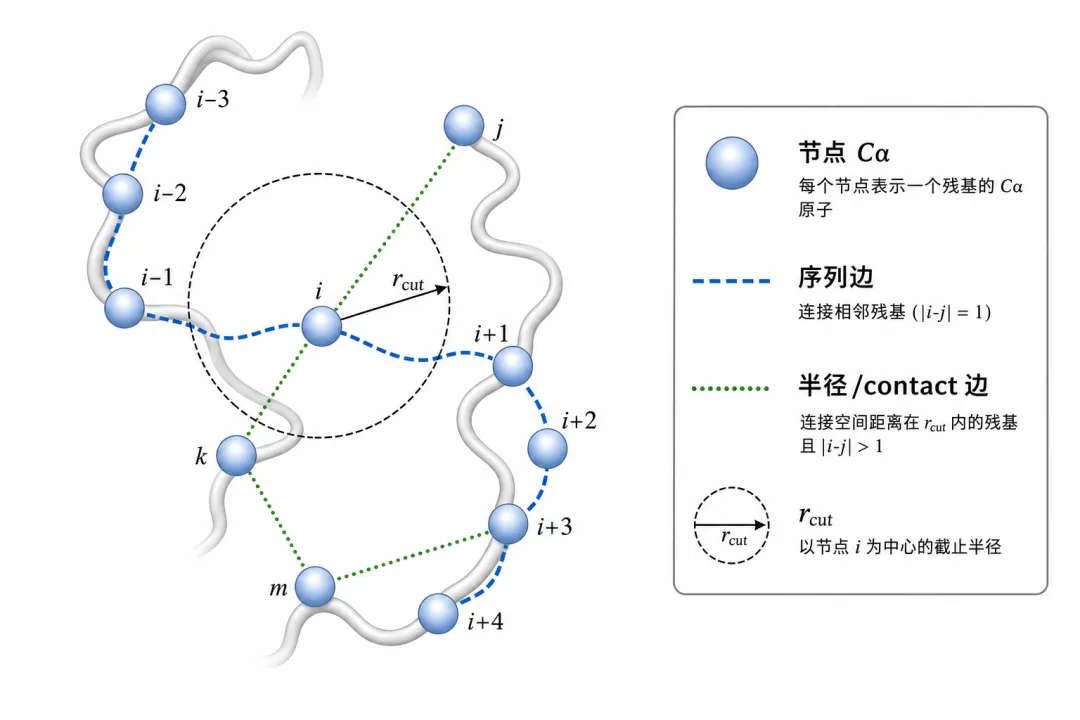 序列边 + 半径/contact 边:两种邻接来源
图 3(科普示意):蛋白残基图常同时使用序列邻接与空间邻接。
6.1 序列边(化学拓扑先验)
相邻残基 与 连无向边(实现上双向各一条):
defsequential_edges(num_nodes: int) -> torch.Tensor:
if num_nodes < 2:
return torch.empty((2, 0), dtype=torch.long)
    src = torch.arange(0, num_nodes - 1)
    dst = src + 1
    edge_index = torch.stack([
        torch.cat([src, dst]),
        torch.cat([dst, src]),
    ], dim=0)
return edge_index  # [2, 2*(N-1)]
6.2 半径图(空间接触)
当 时连边(Å 单位,常用 残基级、全原子更短):
from torch_geometric.nn import radius_graph

pos = torch.from_numpy(table["pos"])  # [N, 3]
edge_radius = radius_graph(
    pos, r=10.0, batch=None, loop=False, max_num_neighbors=64
)
# edge_radius: [2, E_r]
也可用 torch_geometric.nn.knn_graph(pos, k=30) 控制每节点邻居数上界。
6.3 合并边并去重
defmerge_edges(*edge_indices: torch.Tensor) -> torch.Tensor:
    edge_index = torch.cat(edge_indices, dim=1)          # [2, E_all]
# 无向边去重:排序后 unique
    edge_index = edge_index[:, edge_index[0].sort()[1]]
    uniq = torch.unique(edge_index, dim=1)
return uniq
6.4 边特征 edge_attr(可选)
defedge_length_attr(pos: torch.Tensor, edge_index: torch.Tensor) -> torch.Tensor:
    row, col = edge_index
    diff = pos[row] - pos[col]
    dist = torch.linalg.norm(diff, dim=1, keepdim=True)   # [E, 1]
return dist
序列边可附加 ****(序列距离);空间边以 为主。带方向的模型还会用单位向量 (等变 GNN)。
7. 步骤 ⑤:组装 torch_geometric.data.Data
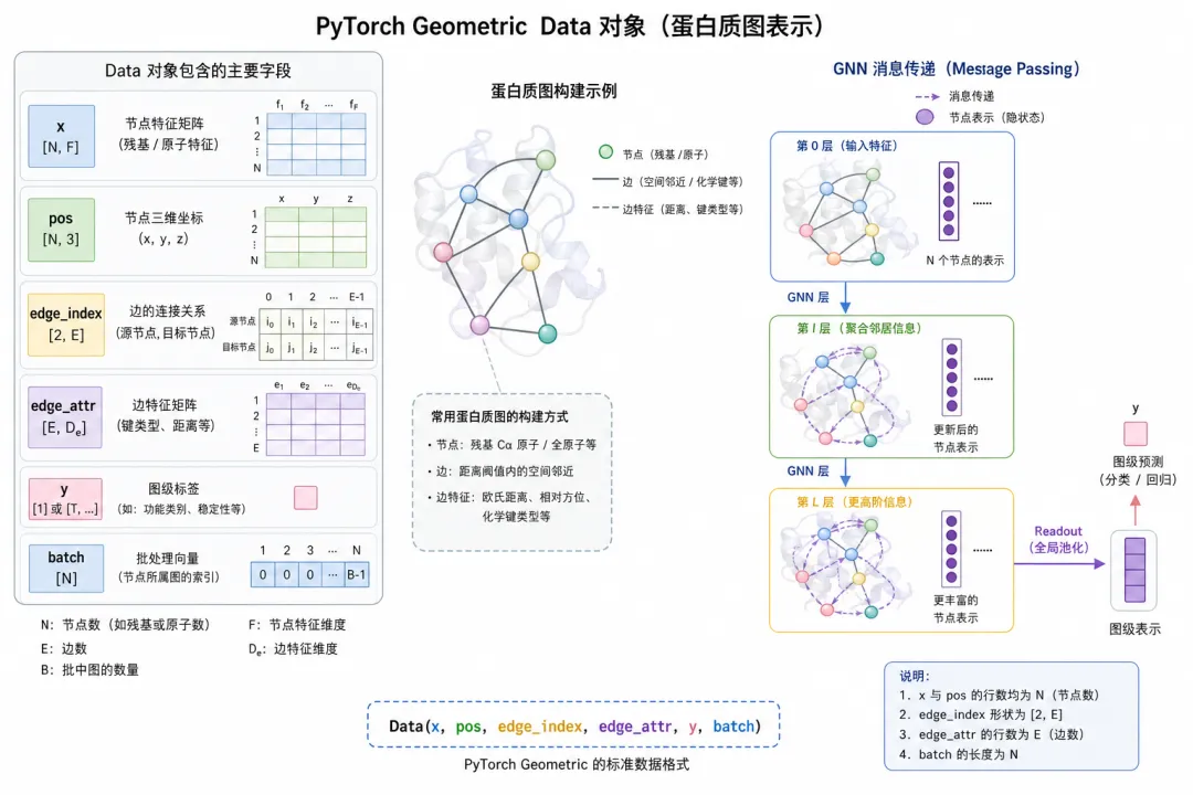 PyG Data 各字段与 GNN 的对应关系
图 4(科普示意):Data 是单张图的「容器」;forward 时由 GNNConv 读 x 与 edge_index。
from torch_geometric.data import Data

defstructure_to_pyg_data(pdb_path: str, chain_id: str = "A") -> Data:
    table = extract_ca_table(pdb_path, chain_id=chain_id)
    pos = torch.from_numpy(table["pos"]).float()
    x = build_node_features(table)
    e_seq = sequential_edges(pos.size(0))
    e_rad = radius_graph(pos, r=10.0, loop=False, max_num_neighbors=64)
    edge_index = merge_edges(e_seq, e_rad)
    edge_attr = edge_length_attr(pos, edge_index)

    data = Data(
        x=x,                   # [N, F] 节点特征
        pos=pos,               # [N, 3] 坐标(几何 GNN / 可视化)
        edge_index=edge_index, # [2, E]
        edge_attr=edge_attr,   # [E, 1]
        num_nodes=pos.size(0),
    )
# 图级标签示例:data.y = torch.tensor([1.0])  # 活性、稳定性等
return data
7.1 Data 与数学对象对照
| |
|---|
data.x | |
data.pos | |
data.edge_index | |
data.edge_attr | |
data.y | |
data.batch | |
8. 批训练:多蛋白如何拼成一批
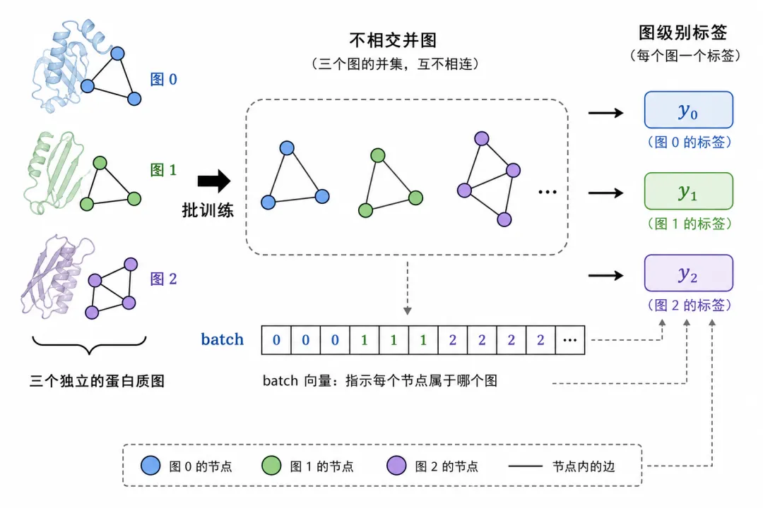 三张蛋白图拼成不相交并图,batch 向量区分图 ID
图 5(科普示意):PyG 的 DataLoader 会把多张图并成一个大图(节点不相连),用 batch 向量区分。
from torch_geometric.data import DataLoader
from torch_geometric.nn import global_mean_pool, GCNConv

classProteinGCN(torch.nn.Module):
def__init__(self, in_dim: int, hidden: int = 128):
        super().__init__()
        self.conv1 = GCNConv(in_dim, hidden)
        self.conv2 = GCNConv(hidden, hidden)
        self.lin = torch.nn.Linear(hidden, 1)

defforward(self, data):
        h = data.x.relu()
        h = self.conv1(h, data.edge_index).relu()
        h = self.conv2(h, data.edge_index)
        hg = global_mean_pool(h, data.batch)   # [B, hidden]
return self.lin(hg).squeeze(-1)         # 图级回归示例

paths = ["1abc.pdb", "2def.pdb", "3ghi.pdb"]
dataset = [structure_to_pyg_data(p) for p in paths]
loader = DataLoader(dataset, batch_size=8, shuffle=True)

for batch in loader:
# batch.x: [N_total, F]; batch.batch: [N_total], 取值 0..B-1
    pred = model(batch)
Dataset 模式:把 structure_to_pyg_data 放进 torch_geometric.data.Dataset 子类,在 get(idx) 里惰性解析 PDB,避免一次性载入万级结构。
9. 数据结构总览(速查表)
| | |
|---|
| | |
| Residue | res["CA"].coord |
| pos[i] | |
| edge_index[:, e] | edge_index[0,e] -> edge_index[1,e] |
| Data | data.num_nodes == data.x.size(0) |
| Batch | data.batch[i] |
索引一致性:edge_index 中的值必须在 内;合并多源边后建议 torch.unique;过滤低 pLDDT 残基后要同步删 pos/x 的行并重映射边。
10. 蛋白结构编码的常见建模选择
编码的最终产物是:**在保留几何与序列先验的图上,每个残基有一个初始嵌入 **;后续 GNN 层通过消息传递得到 、,用于活性预测、界面识别、突变效应等下游任务。
11. 最小可运行依赖
pip install biopython numpy torch torch-geometric
# PyG 安装若遇 CUDA 版本问题,见官方 wheel 说明
项目目录示例
├── data/
│   └── 1CRN.pdb
├── graph/
│   └── build_protein_graph.py   # 本文 extract / structure_to_pyg_data
└── train/
    └── train_gcn.py             # DataLoader + GCN
12. 小结
用 Python 做蛋白结构的 GNN 编码,本质是 「结构文件 → 残基表 → 图张量 → PyG Data」。BioPython(或 biotite)负责语义解析,NumPy/PyTorch 负责数值表,edge_index 负责关系,PyG 负责与 GNN 层对接。记住三张图:对象树(便于筛链筛残基)、坐标表 pos(几何与构图)、特征表 x(化学与统计),再记住两种边:序列与空间,就能把文献里的蛋白 GNN 数据管线读懂、写通。
参考文献与延伸阅读
- BioPython Tutorial — Structure section
- PyTorch Geometric — Creating Your Own Datasets
- Hamelryck & Manderick, PDB parser and structure class (BioPython PDB).
 10个月宝宝每天需要喝多少奶粉?
