当前位置：首页>python>Nature 期刊图复现 | Python 实现多组别个体散点图、中位数线与饼图组合

Nature 期刊图复现 | Python 实现多组别个体散点图、中位数线与饼图组合

2026-09-10 17:14:10

来源论文

论文地址：

https://www.nature.com/articles/s41586-025-09653-0

论文题目：

Mapping Plasmodium transitions and interactions in the Anopheles female

复现图片

常用于全面阐明各组定量数据的分布规律。上方利用抖动散点与中位数线表征连续变量的离散度与集中趋势；下方轴外对齐嵌入微型饼图与元数据表，同步揭示群体样本量与阳性率。该设计有效融合了微观个体分布与宏观群体比例，显著提升了学术图表的信息高密度输出。

配色方案

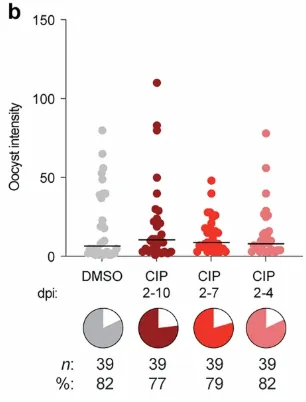
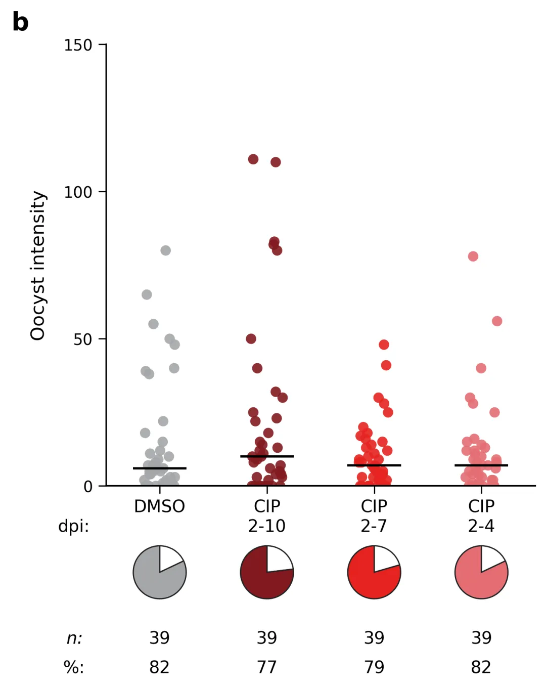
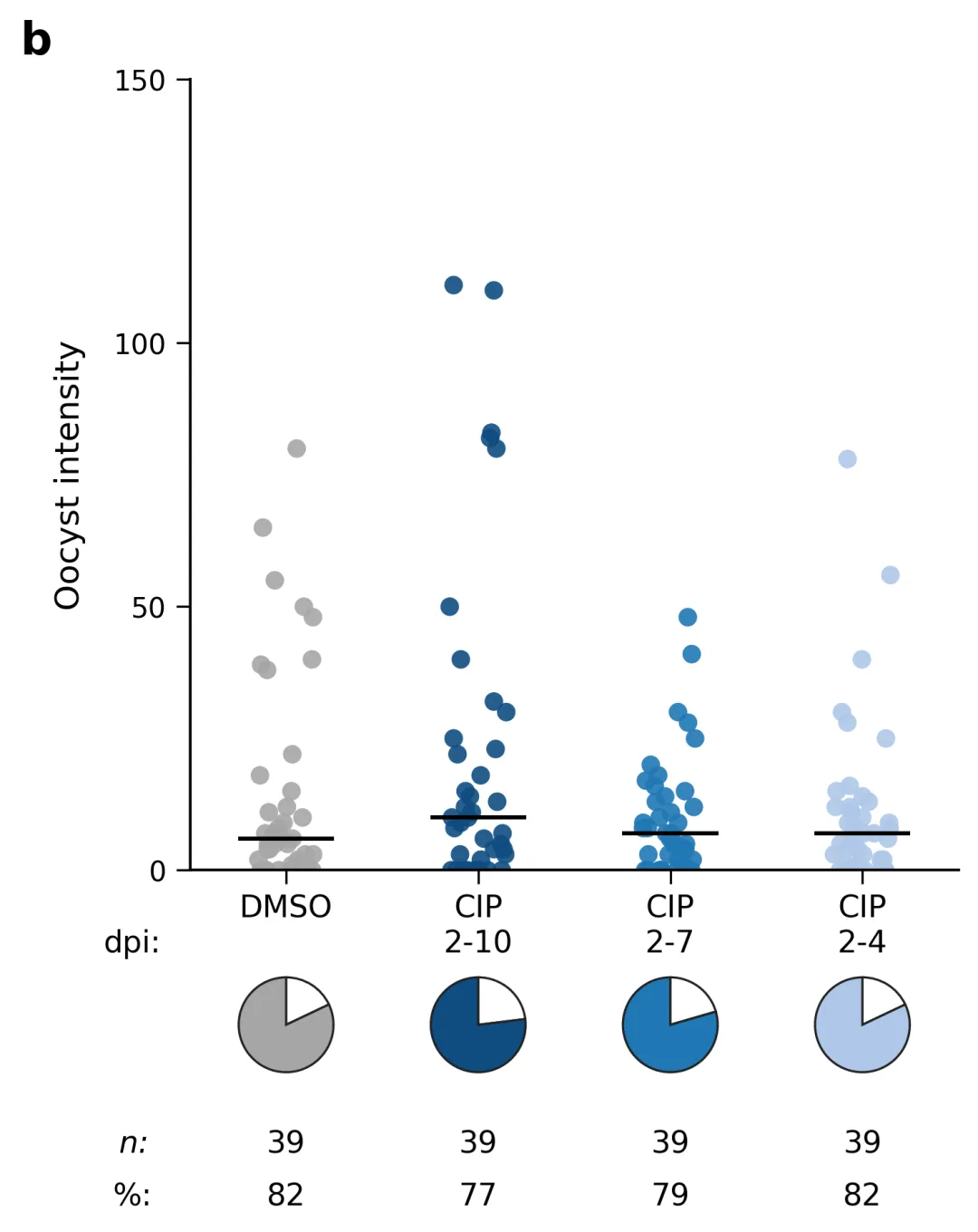
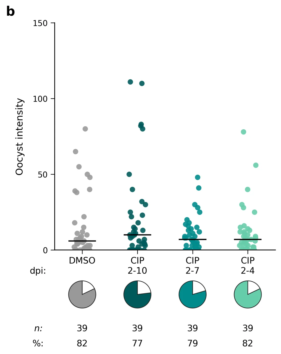
color_schemes = {        1: {('DMSO', ''): '#A5A6A9', ('CIP', '2-10'): '#82191F', ('CIP', '2-7'): '#E52320', ('CIP', '2-4'): '#E46E73'},  # 方案1: Nature 经典红灰渐变系列        2: {('DMSO', ''): '#A6A6A6', ('CIP', '2-10'): '#0F4C81', ('CIP', '2-7'): '#1F77B4', ('CIP', '2-4'): '#AEC7E8'},  # 方案2: Cell 经典蓝灰渐变系列        3: {('DMSO', ''): '#999999', ('CIP', '2-10'): '#005A5B', ('CIP', '2-7'): '#008B8B', ('CIP', '2-4'): '#66CDAA'},  # 方案3: Science 经典青绿渐变系列        4: {('DMSO', ''): '#8A8B8C', ('CIP', '2-10'): '#104E8B', ('CIP', '2-7'): '#B22222', ('CIP', '2-4'): '#FF8C00'},  # 方案4: NEJM 高对比度经典多色        5: {('DMSO', ''): '#7F8C8D', ('CIP', '2-10'): '#800020', ('CIP', '2-7'): '#4A235A', ('CIP', '2-4'): '#D35400'},  # 方案5: Lancet 深调典雅传统多色        6: {('DMSO', ''): '#B0B0B0', ('CIP', '2-10'): '#A0522D', ('CIP', '2-7'): '#FF7F50', ('CIP', '2-4'): '#FFD700'},  # 方案6: Nature Communications 暖色调多色        7: {('DMSO', ''): '#9E9E9E', ('CIP', '2-10'): '#1A365D', ('CIP', '2-7'): '#2F855A', ('CIP', '2-4'): '#48BB78'},  # 方案7: EMBO Journal 蓝绿渐变系列        8: {('DMSO', ''): '#A0A0A0', ('CIP', '2-10'): '#4B0082', ('CIP', '2-7'): '#8A2BE2', ('CIP', '2-4'): '#D8BFD8'},  # 方案8: JCO 优雅紫罗兰渐变系列        9: {('DMSO', ''): '#888888', ('CIP', '2-10'): '#002060', ('CIP', '2-7'): '#C00000', ('CIP', '2-4'): '#00B050'},  # 方案9: PNAS 标准高饱和对比色        10: {('DMSO', ''): '#95A5A6', ('CIP', '2-10'): '#2C3E50', ('CIP', '2-7'): '#E67E22', ('CIP', '2-4'): '#F39C12'},  # 方案10: ACS 珊瑚橙青灰对比色        11: {('DMSO', ''): '#B2B2B2', ('CIP', '2-10'): '#556B2F', ('CIP', '2-7'): '#8B814C', ('CIP', '2-4'): '#CDCDC1'},  # 方案11: Nature Medicine 质感大地色系        12: {('DMSO', ''): '#909090', ('CIP', '2-10'): '#4A148C', ('CIP', '2-7'): '#8E24AA', ('CIP', '2-4'): '#F06292'},  # 方案12: Science Signaling 迷幻紫粉渐变        13: {('DMSO', ''): '#7A7A7A', ('CIP', '2-10'): '#5B0E2D', ('CIP', '2-7'): '#9E1030', ('CIP', '2-4'): '#FFAA91'},  # 方案13: Blood 杂志强感染血红调        14: {('DMSO', ''): '#AAAAAA', ('CIP', '2-10'): '#0B3C5D', ('CIP', '2-7'): '#328CC1', ('CIP', '2-4'): '#D9B310'},  # 方案14: Circulation 商务深海金蓝配        15: {('DMSO', ''): '#8C8C8C', ('CIP', '2-10'): '#A04000', ('CIP', '2-7'): '#D35400', ('CIP', '2-4'): '#EDBB99'},  # 方案15: Gastroenterology 温暖红褐渐变        16: {('DMSO', ''): '#A3A3A3', ('CIP', '2-10'): '#004D40', ('CIP', '2-7'): '#00796B', ('CIP', '2-4'): '#00BFA5'},  # 方案16: Immunity 晶莹深翠绿渐变        17: {('DMSO', ''): '#616161', ('CIP', '2-10'): '#212121', ('CIP', '2-7'): '#D50000', ('CIP', '2-4'): '#FF6D00'},  # 方案17: Cancer Cell 高警示红黑对比        18: {('DMSO', ''): '#A1A1A1', ('CIP', '2-10'): '#311B92', ('CIP', '2-7'): '#4527A0', ('CIP', '2-4'): '#B39DDB'},  # 方案18: Journal of Virology 深空紫调        19: {('DMSO', ''): '#9E9E9E', ('CIP', '2-10'): '#1B5E20', ('CIP', '2-7'): '#2E7D32', ('CIP', '2-4'): '#A5D6A7'},  # 方案19: Nature Biotechnology 生态纯绿渐变        20: {('DMSO', ''): '#757575', ('CIP', '2-10'): '#0D47A1', ('CIP', '2-7'): '#1565C0', ('CIP', '2-4'): '#90CAF9'}   # 方案20: Classic Navy 经典海军蓝渐变    }

完整代码

import osimport numpy as npimport pandas as pdimport matplotlib.pyplot as pltdef main():    # 1. 自动创建 “图表” 文件夹    output_dir = "图表"    os.makedirs(output_dir, exist_ok=True)    # 2. 自动读取当前目录下的 data.xlsx    excel_file = "data.xlsx"    if not os.path.exists(excel_file):        raise FileNotFoundError(f"未在当前目录下找到 {excel_file} 文件，请先运行 generate_data.py 生成数据！")    df = pd.read_excel(excel_file)    print(f"成功从 {excel_file} 读取数据，正在绘制图表...")    # 3. 定义严格对应的组别顺序与主流期刊专业科研配色方案字典    group_order = [        ('DMSO', ''),        ('CIP', '2-10'),        ('CIP', '2-7'),        ('CIP', '2-4')    ]    color_schemes = {        1: {('DMSO', ''): '#A5A6A9', ('CIP', '2-10'): '#82191F', ('CIP', '2-7'): '#E52320', ('CIP', '2-4'): '#E46E73'},  # 方案1: Nature 经典红灰渐变系列    }    # 当前默认选择方案1    colors = color_schemes[1]    # 4. 初始化画布    fig, ax = plt.subplots(figsize=(5.5, 7.2))    plt.subplots_adjust(bottom=0.35, left=0.2, right=0.9, top=0.9)    np.random.seed(42)    # 5. 遍历各组绘制主散点图与中位数线    for idx, (grp, dpi) in enumerate(group_order):        if pd.isna(dpi) or dpi == '':            sub_df = df[(df['Group'] == grp) & (df['DPI'].isna() | (df['DPI'] == ''))]        else:            sub_df = df[(df['Group'] == grp) & (df['DPI'].astype(str) == str(dpi))]        vals = sub_df['Oocyst_Intensity'].values        jitter = np.random.uniform(-0.15, 0.15, size=len(vals))        x_pos = idx + jitter        color = colors[(grp, dpi)]        ax.scatter(x_pos, vals, color=color, s=45, alpha=0.9, edgecolors='none', zorder=2)        median_val = np.median(vals) if len(vals) > 0 else 0        ax.hlines(median_val, idx - 0.25, idx + 0.25, colors='black', linewidth=1.5, zorder=3)    # 6. 美化主图坐标轴    ax.set_xlim(-0.5, 3.5)    ax.set_ylim(0, 150)    ax.set_ylabel('Oocyst intensity', fontsize=12, labelpad=10)    ax.set_xticks(range(4))    ax.set_xticklabels([g[0] for g in group_order], fontsize=11)    ax.set_yticks([0, 50, 100, 150])    ax.spines['top'].set_visible(False)    ax.spines['right'].set_visible(False)    ax.spines['left'].set_linewidth(1)    ax.spines['bottom'].set_linewidth(1)    ax.tick_params(direction='out', length=5)    # 在左上角添加序号b (使用 transAxes 确保相对于轴线框左上角对齐)    ax.text(-0.18, 1.02, 'b', transform=ax.transAxes, fontsize=16, fontweight='bold', va='bottom', ha='right')    # 7. 动态计算并在下方绘制文本行与饼图    ax.text(-0.8, -14, 'dpi:', ha='center', va='center', fontsize=11)    ax.text(-0.8, -52, r'$n$:', ha='center', va='center', fontsize=11, style='italic')    ax.text(-0.8, -62, r'%:', ha='center', va='center', fontsize=11)    main_pos = ax.get_position()    for idx, (grp, dpi) in enumerate(group_order):        if pd.isna(dpi) or dpi == '':            sub_df = df[(df['Group'] == grp) & (df['DPI'].isna() | (df['DPI'] == ''))]        else:            sub_df = df[(df['Group'] == grp) & (df['DPI'].astype(str) == str(dpi))]        vals = sub_df['Oocyst_Intensity'].values        n_total = len(vals)        n_infected = np.sum(vals > 0)        pct_infected = (n_infected / n_total) * 100 if n_total > 0 else 0        ax.text(idx, -14, str(dpi) if (not pd.isna(dpi) and dpi != '') else '', ha='center', va='center', fontsize=11)        ax.text(idx, -52, f"{n_total}", ha='center', va='center', fontsize=11)        ax.text(idx, -62, f"{int(round(pct_infected))}", ha='center', va='center', fontsize=11)        trans = ax.get_xaxis_transform()        pixel_pos = trans.transform((idx, 0))        fig_pos = fig.transFigure.inverted().transform(pixel_pos)        pie_size = 0.095        pie_x = fig_pos[0] - pie_size / 2        pie_y = main_pos.y0 - 0.155        pie_ax = fig.add_axes([pie_x, pie_y, pie_size, pie_size])        pie_ax.pie(            [100 - pct_infected, pct_infected],            colors=['#FFFFFF', colors[(grp, dpi)]],            startangle=90,            counterclock=False,            wedgeprops={'edgecolor': '#222222', 'linewidth': 0.8}        )        pie_ax.axis('equal')    # 8. 保存高质量 PNG    output_path = os.path.join(output_dir, "sv_distribution_3d.png")    plt.savefig(output_path, dpi=300, bbox_inches='tight')    plt.close()    print(f"绘图成功！图表已完美保存至: {output_path}")if __name__ == "__main__":    main()