搞遥感 GIS 的朋友,拿到一套无人机多光谱 + 热红外数据,想做个地物分类加温度分析,打开 ENVI 点半天,步骤多到记不住,换个数据又得重来一遍,鼠标都快点冒烟了。
今天直接给大家上一套 Python 懒人套餐,从 4 类地物自动分类,到热红外温度对齐出图,代码复制过去改个路径就能跑,告别繁琐的菜单操作。
一、4 类地物分类:阈值法,不用训练样本
很多人一上来就想搞机器学习监督分类,其实简单的农田、城市场景下,经验阈值法才是性价比之王 —— 不用标样本,不用训模型,几行代码直接出结果。
我们用到 4 个多光谱波段:红光、绿光、近红外、红边,靠两个核心指标打天下:
- NDVI 归一化植被指数
- :植被的专属身份证,植被近红外反射高、红光反射低,一算一个准
- 波段平均亮度
分类逻辑简单粗暴,按优先级判断:
- NDVI < 0 + 低亮度 + 近红外值低 → 水体
- 非植被非水体,亮度≥1000 → 不透水面(道路、建筑)
看看分类效果,研究区以绿色的农田植被为主,橙色的田埂裸地穿插其中,红色的建筑道路边界清晰,应付课程作业、项目初筛完全够用。
核心处理代码如下,用 rasterio 分块读取影像,再大的 tif 也不怕爆内存:
# 计算核心指数ndvi = (nir - red) / (nir + red + 1e-9)bright = (red + green + nir + rededge) / 4.0# 分类判别water = valid & (ndvi < 0.0) & (bright < 700.0) & (nir < 900.0)veg = valid & (ndvi >= 0.25)impervious = valid & (~veg) & (~water) & (bright >= 1000.0)bare_soil = valid & (~veg) & (~water) & (~impervious)
二、地表温度分析:对齐是第一步,不然全白搭
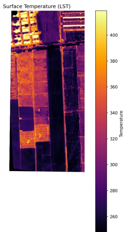
很多新手做地物温度统计最容易踩的坑:多光谱分类图和热红外温度图分辨率、投影、范围全不一样,像素根本对不上,算出来的平均温度纯纯无效数据。所以第一步必须做空间对齐:把热红外温度数据重投影到和分类图完全一致的栅格网格上,保证每个像素一一对应。我们用双线性插值重采样,适合温度这种连续型数据,过渡自然不会出现锯齿。出图效果如上,色带越亮温度越高,肉眼就能看出地物和温度的对应规律。对齐完成后,我们直接按地物类别做掩膜统计,得到各类的温度均值:别慌,这是原始热红外数据的温度反演参数没调好,不是咱们代码的锅。正常的热环境规律肯定是不透水面温度最高、水体温度最低,大家自己实操的时候,记得先校验热红外数据的辐射定标、大气校正和比辐射率参数,咱们这套流程是方法框架通用,数值对错全看输入数据。热红外数据重投影对齐reproject( source=rasterio.band(src, 1), destination=dest, src_transform=src.transform, src_crs=src.crs, dst_transform=match_profile['transform'], dst_crs=match_profile['crs'], resampling=Resampling.bilinear)
地物分类代码:
import numpy as npimport rasterioimport matplotlib.pyplot as pltfrom matplotlib.patches import Patchinput_files = { 'red': 'result_Red.tif', 'green': 'result_Green.tif', 'nir': 'result_NIR.tif', 'rededge': 'result_RedEdge.tif',}output_tif = 'landcover_4class.tif'output_png = 'landcover_4class.png'# Class codes:# 0 = background / no data# 1 = Vegetation# 2 = Bare soil# 3 = Impervious surface# 4 = Waterclass_labels = { 1: 'Vegetation', 2: 'Bare soil', 3: 'Impervious surface', 4: 'Water',}class_colors = { 0: (0, 0, 0), 1: (44, 160, 44), 2: (237, 125, 49), 3: (178, 34, 34), 4: (31, 119, 180),}with rasterio.open(input_files['red']) as src_red: profile = src_red.profile.copy() width = src_red.width height = src_red.height profile.update(count=1, dtype=rasterio.uint8, compress='lzw', nodata=0) with rasterio.open(output_tif, 'w', **profile) as dst: classification = np.zeros((height, width), dtype=np.uint8) with rasterio.open(input_files['green']) as src_green, \ rasterio.open(input_files['nir']) as src_nir, \ rasterio.open(input_files['rededge']) as src_rededge: for _, window in src_red.block_windows(1): red = src_red.read(1, window=window).astype(np.float32) green = src_green.read(1, window=window).astype(np.float32) nir = src_nir.read(1, window=window).astype(np.float32) rededge = src_rededge.read(1, window=window).astype(np.float32) ndvi = (nir - red) / (nir + red + 1e-9) bright = (red + green + nir + rededge) / 4.0 valid = np.isfinite(ndvi) tile = np.zeros(red.shape, dtype=np.uint8) water = valid & (ndvi < 0.0) & (bright < 700.0) & (nir < 900.0) veg = valid & (ndvi >= 0.25) impervious = valid & (~veg) & (~water) & (bright >= 1000.0) bare_soil = valid & (~veg) & (~water) & (~impervious) tile[bare_soil] = 2 tile[impervious] = 3 tile[veg] = 1 tile[water] = 4 dst.write(tile, 1, window=window) classification[window.row_off:window.row_off + window.height, window.col_off:window.col_off + window.width] = tileprint(f'Wrote classification raster: {output_tif}')rgb = np.zeros((height, width, 3), dtype=np.uint8)for cls, color in class_colors.items(): rgb[classification == cls] = colorfig, ax = plt.subplots(figsize=(12, 10))ax.imshow(rgb)ax.axis('off')legend_handles = [Patch(facecolor=np.array(class_colors[cls]) / 255.0, label=label) for cls, label in class_labels.items()]ax.legend(handles=legend_handles, loc='lower right', fontsize='large', framealpha=0.85)ax.set_title('4-class land cover map: Vegetation, Bare soil, Impervious surface, Water', fontsize=16)fig.tight_layout(pad=0.5)fig.savefig(output_png, dpi=150, bbox_inches='tight')plt.close(fig)print(f'Wrote classification image: {output_png}')
地表温度代码:
#!/usr/bin/env python3"""Generate surface temperature PNG map and aligned TIFF from raster outputs."""import osimport matplotlibmatplotlib.use('Agg')import matplotlib.pyplot as pltimport numpy as npimport rasteriofrom rasterio.warp import reproject, Resamplingdef load_surface_temperature(lst_path, match_profile): """加载地表温度影像,并重投影对齐到参考栅格的空间网格""" with rasterio.open(lst_path) as src: dest = np.full((match_profile['height'], match_profile['width']), np.nan, dtype=np.float32) reproject( source=rasterio.band(src, 1), destination=dest, src_transform=src.transform, src_crs=src.crs, dst_transform=match_profile['transform'], dst_crs=match_profile['crs'], resampling=Resampling.bilinear, src_nodata=src.nodata, dst_nodata=np.nan, ) return destdef save_temperature_map(lst, output_path): """渲染并保存地表温度PNG分布图""" valid = np.isfinite(lst) if np.count_nonzero(valid) == 0: raise RuntimeError('No valid temperature pixels found.') vmin = float(np.nanpercentile(lst[valid], 2)) vmax = float(np.nanpercentile(lst[valid], 98)) fig, ax = plt.subplots(figsize=(10, 8)) im = ax.imshow(lst, cmap='inferno', vmin=vmin, vmax=vmax) ax.set_title('Surface Temperature (LST)') ax.axis('off') cbar = fig.colorbar(im, ax=ax, fraction=0.046, pad=0.04) cbar.set_label('Temperature') fig.tight_layout() fig.savefig(output_path, dpi=150) plt.close(fig)def save_surface_temperature_tif(lst, profile, output_path): """保存对齐后的地表温度TIFF文件(带LZW压缩)""" out_profile = profile.copy() out_profile.update({ 'count': 1, 'dtype': 'float32', 'nodata': np.nan, 'compress': 'lzw' }) with rasterio.open(output_path, 'w', **out_profile) as dst: arr = lst.astype(np.float32) arr[~np.isfinite(arr)] = out_profile['nodata'] dst.write(arr, 1)def main(): os.makedirs('figures', exist_ok=True) # 参考栅格路径:用于提供目标空间坐标系、分辨率、范围(可替换为任意匹配的栅格文件) reference_path = r'D:\data\MultiSpectral\output_landcover_test5\Landcover_Class_20260708.tif' lst_path = r'D:\data\MultiSpectral\0708s\TIR_LST20260708.tif' # 读取参考栅格的空间元数据 with rasterio.open(reference_path) as src: reference_profile = src.profile # 加载并对齐地表温度 lst = load_surface_temperature(lst_path, reference_profile) temp_out = os.path.join('figures', 'surface_temperature_map.png') temp_tif_out = os.path.join('figures', 'surface_temperature_aligned.tif') save_temperature_map(lst, temp_out) save_surface_temperature_tif(lst, reference_profile, temp_tif_out) print('Generated:', temp_out) print('Generated:', temp_tif_out)if __name__ == '__main__': main()
三、三步上手,直接跑通
装依赖
:一行命令搞定环境
pip install numpy rasterio matplotlib
改路径:把两个脚本里的输入文件路径,替换成你自己的多光谱波段、热红外温度文件路径
运行脚本:依次执行分类脚本和温度脚本,坐等输出结果
最后说两句
代码逻辑很简单,大家可以根据自己的研究区调整 NDVI、亮度的阈值,分类精度还能再提一档。觉得有用的朋友别忘了点赞收藏,下次找代码不迷路。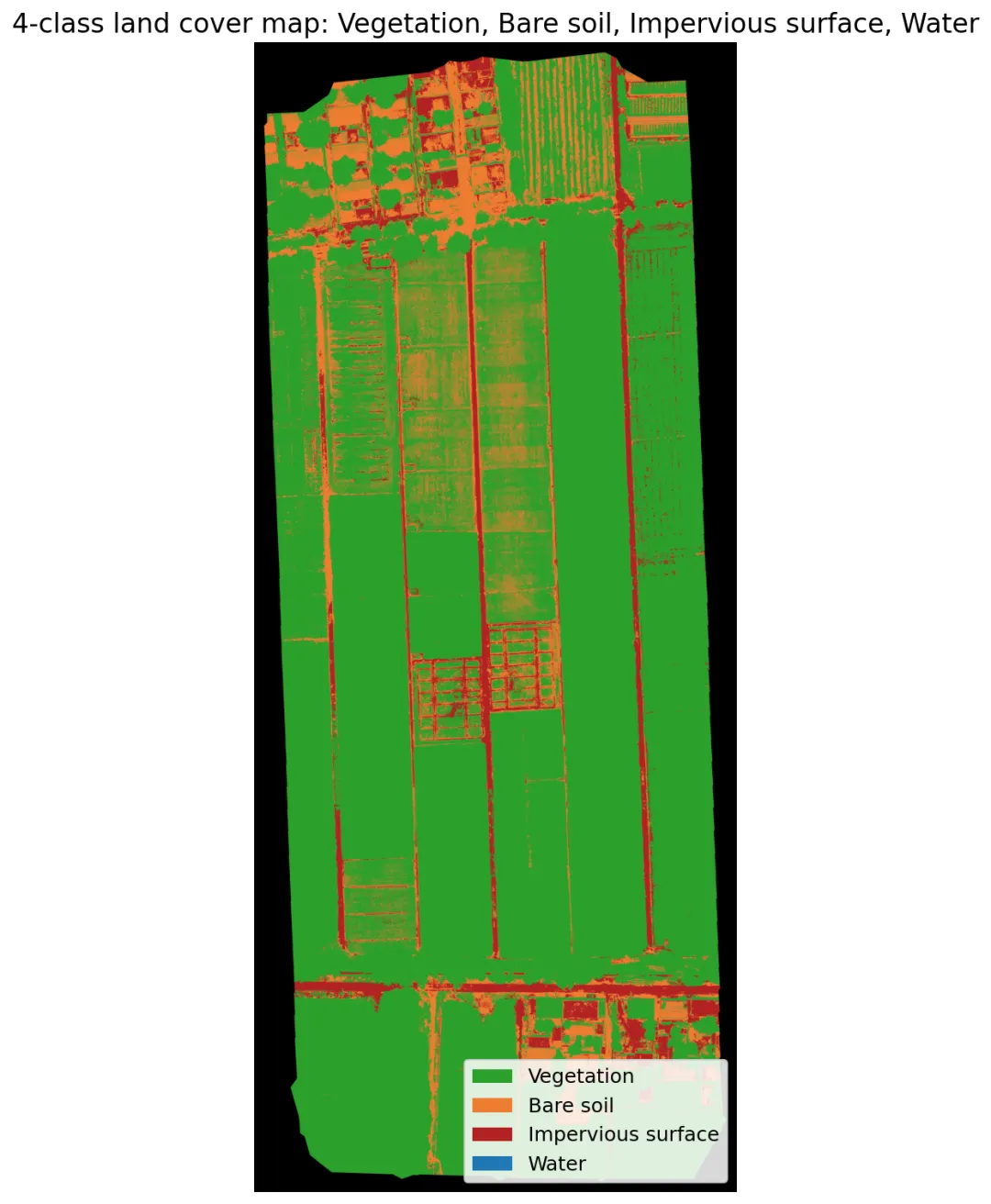
 10个月宝宝每天需要喝多少奶粉?