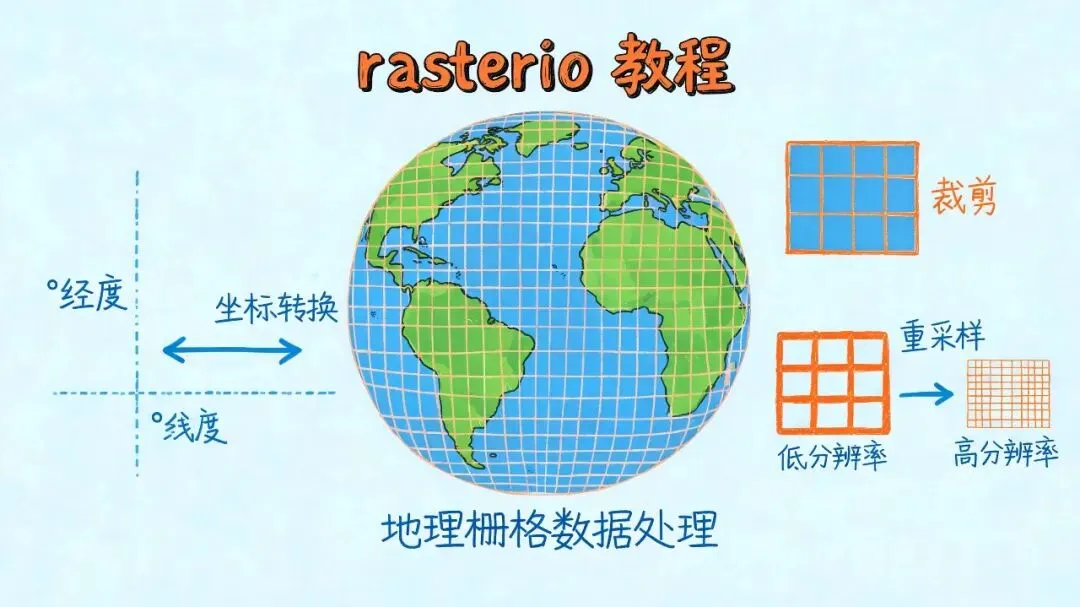
气象数据常以栅格格式存储,如卫星影像、再分析数据的 GeoTIFF 文件。rasterio 是处理这类数据的专业工具。
今天这篇文章,带你掌握用 rasterio 处理气象栅格数据的核心方法,并学习如何从镜像地球开放平台获取 GeoTIFF 格式的数据。
前言:从哪里获取 GeoTIFF 气象数据?
rasterio 最擅长处理 GeoTIFF 格式的栅格数据。镜像地球开放平台提供了图层产品 API,可直接获取 GeoTIFF 格式的栅格数据:
使用镜像地球图层 API
import requestsimport rasteriofrom rasterio.io import MemoryFileimport io# 获取 HRES 图层瓦片数据(GeoTIFF 格式)layer_url = "https://api.mirror-earth.com/v1/layer/hres/webgl"params = { "layer": "temperature_2m", "time": "2024-07-29T12:00", "bbox": "110,30,120,40", # xmin,ymin,xmax,ymax "apikey": "your_api_key"}response = requests.get(layer_url, params=params)if response.status_code == 200: # 直接在内存中打开 GeoTIFF with MemoryFile(response.content) as memfile: with memfile.open() as src: print(f"坐标系: {src.crs}") print(f"边界: {src.bounds}") print(f"尺寸: {src.width} x {src.height}") # 读取数据 data = src.read(1) print(f"温度范围: {data.min():.2f}K 至 {data.max():.2f}K")
镜像地球可获取的 GeoTIFF 数据类型
| | | |
|---|
| HRES 图层 | | | |
| GFS 图层 | | | |
| 风场粒子 | | | |
| 卫星云图 | | | |
| 雷达拼图 | | | |
一、基础读取
1.1 读取 GeoTIFF 文件
import rasteriofrom rasterio.plot import showimport matplotlib.pyplot as plt# 打开文件with rasterio.open('weather_tiff.tif') as src: # 查看文件信息 print(src.profile) # 读取数据 data = src.read(1) # 读取第一个波段 # 查看数据形状 print(f"数据形状: {data.shape}") # 查看坐标系统 print(f"坐标系: {src.crs}") # 查看变换参数 print(f"变换参数: {src.transform}")# 显示数据plt.figure(figsize=(10, 8))plt.imshow(data, cmap='RdYlBu_r')plt.colorbar(label='温度 (℃)')plt.title('温度分布')plt.show()
1.2 获取元数据
with rasterio.open('weather_tiff.tif') as src: # 文件尺寸 height = src.height width = src.width bands = src.count # 坐标边界 bounds = src.bounds # (left, bottom, right, top) # 分辨率 resolution = src.res # (x_resolution, y_resolution) # 数据类型 dtype = src.dtypes[0] print(f"尺寸: {height} x {width}") print(f"波段数: {bands}") print(f"边界: {bounds}") print(f"分辨率: {resolution}") print(f"数据类型: {dtype}")
二、坐标转换
2.1 像素坐标转地理坐标
import rasteriodef pixel_to_geo(src, row, col): """像素坐标转地理坐标""" # 获取转换矩阵 transform = src.transform # 转换坐标 lon, lat = transform * (col, row) return lon, lat# 使用with rasterio.open('weather_tiff.tif') as src: # 图像中心点 center_row = src.height // 2 center_col = src.width // 2 center_lon, center_lat = pixel_to_geo(src, center_row, center_col) print(f"中心点: ({center_lon:.4f}, {center_lat:.4f})")
2.2 地理坐标转像素坐标
def geo_to_pixel(src, lon, lat): """地理坐标转像素坐标""" # 获取逆变换矩阵 transform = ~src.transform # 转换坐标 col, row = transform * (lon, lat) return int(round(row)), int(round(col))# 使用with rasterio.open('weather_tiff.tif') as src: # 北京坐标 beijing_lon, beijing_lat = 116.4, 39.9 beijing_row, beijing_col = geo_to_pixel(src, beijing_lon, beijing_lat) print(f"北京像素坐标: ({beijing_row}, {beijing_col})")
2.3 坐标系转换
from rasterio.warp import calculate_default_transform, reproject, Resamplingfrom rasterio.crs import CRSdef reproject_raster(input_path, output_path, target_crs): """重投影栅格数据""" with rasterio.open(input_path) as src: # 计算重投影参数 transform, width, height = calculate_default_transform( src.crs, target_crs, src.width, src.height, *src.bounds ) # 设置输出参数 kwargs = src.meta.copy() kwargs.update({ 'crs': target_crs, 'transform': transform, 'width': width, 'height': height }) # 重投影 with rasterio.open(output_path, 'w', **kwargs) as dst: for i in range(1, src.count + 1): reproject( source=rasterio.band(src, i), destination=rasterio.band(dst, i), src_transform=src.transform, src_crs=src.crs, dst_transform=transform, dst_crs=target_crs, resampling=Resampling.nearest )# 使用:从 EPSG:4326 重投影到 EPSG:3857reproject_raster( 'weather_4326.tif', 'weather_3857.tif', CRS.from_epsg(3857))
三、数据裁剪
3.1 按边界框裁剪
from rasterio.windows import Windowfrom rasterio.warp import transform_boundsdef clip_by_bounds(input_path, output_path, bounds): """按边界框裁剪""" with rasterio.open(input_path) as src: # 转换边界框到源坐标系 transformed_bounds = transform_bounds( CRS.from_epsg(4326), # 输入边界框的坐标系 src.crs, *bounds ) # 计算窗口 window = src.window(*transformed_bounds) # 读取裁剪数据 data = src.read(1, window=window) # 转换窗口 transform = src.window_transform(window) # 保存裁剪结果 profile = src.profile profile.update({ 'height': window.height, 'width': window.width, 'transform': transform }) with rasterio.open(output_path, 'w', **profile) as dst: dst.write(data, 1)# 使用:裁剪中国区域china_bounds = (70, 15, 140, 55) # (west, south, east, north)clip_by_bounds('global_weather.tif', 'china_weather.tif', china_bounds)
3.2 按多边形裁剪
from shapely.geometry import box, mappingfrom rasterio.mask import maskdef clip_by_polygon(input_path, output_path, polygon): """按多边形裁剪""" with rasterio.open(input_path) as src: # 裁剪数据 out_image, out_transform = mask(src, [polygon], crop=True) # 更新配置 out_meta = src.meta.copy() out_meta.update({ "driver": "GTiff", "height": out_image.shape[1], "width": out_image.shape[2], "transform": out_transform }) # 保存结果 with rasterio.open(output_path, "w", **out_meta) as dst: dst.write(out_image)# 使用:裁剪北京市beijing_box = box(116.0, 39.5, 117.0, 40.5) # 西、南、东、北beijing_polygon = mapping(beijing_box)clip_by_polygon('china_weather.tif', 'beijing_weather.tif', beijing_polygon)
四、数据处理
4.1 数据统计
import numpy as npdef calculate_statistics(data): """计算栅格数据统计""" return { 'mean': np.nanmean(data), 'std': np.nanstd(data), 'min': np.nanmin(data), 'max': np.nanmax(data), 'median': np.nanmedian(data), 'q25': np.nanpercentile(data, 25), 'q75': np.nanpercentile(data, 75), 'nodata': np.isnan(data).sum() }# 使用with rasterio.open('weather_tiff.tif') as src: data = src.read(1) stats = calculate_statistics(data) print("栅格数据统计:") for key, value in stats.items(): print(f" {key}: {value:.2f}")
4.2 数据分类
def classify_temperature(data, classes=None): """温度分类""" if classes is None: classes = [ (-float('inf'), 273.15), # 严寒 (273.15, 283.15), # 寒冷 (283.15, 293.15), # 温和 (293.15, 303.15), # 炎热 (303.15, float('inf')) # 酷热 ] # 创建分类数组 classified = np.zeros_like(data, dtype=np.int8) # 分类 for i, (lower, upper) in enumerate(classes, 1): mask = (data >= lower) & (data < upper) classified[mask] = i return classified# 使用with rasterio.open('temperature.tif') as src: data = src.read(1) - 273.15 # 转为摄氏度 classified = classify_temperature(data) # 保存分类结果 profile = src.profile profile.update(dtype=rasterio.int8) with rasterio.open('temperature_classified.tif', 'w', **profile) as dst: dst.write(classified, 1)
4.3 数据重采样
from rasterio.warp import reproject, Resamplingdef resample_raster(input_path, output_path, scale_factor): """重采样栅格数据""" with rasterio.open(input_path) as src: # 计算新尺寸 new_height = int(src.height * scale_factor) new_width = int(src.width * scale_factor) # 创建目标数组 data = src.read(1) resampled = np.zeros((new_height, new_width), dtype=data.dtype) # 重投影到新尺寸 from rasterio.warp import calculate_default_transform transform, width, height = calculate_default_transform( src.crs, src.crs, src.width, src.height, *src.bounds, dst_width=new_width, dst_height=new_height ) # 执行重采样 reproject( source=data, destination=resampled, src_transform=src.transform, src_crs=src.crs, dst_transform=transform, dst_crs=src.crs, resampling=Resampling.bilinear ) # 保存结果 profile = src.profile profile.update({ 'height': new_height, 'width': new_width, 'transform': transform }) with rasterio.open(output_path, 'w', **profile) as dst: dst.write(resampled, 1)# 使用:降采样到一半分辨率resample_raster('high_res.tif', 'low_res.tif', scale_factor=0.5)
五、实战案例
5.1 ERA5 栅格数据可视化
import rasterioimport matplotlib.pyplot as pltimport cartopy.crs as ccrsimport cartopy.feature as cfeatureimport numpy as npdef visualize_era5_data(file_path): """可视化镜像地球 ERA5 栅格数据""" with rasterio.open(file_path) as src: # 读取数据 data = src.read(1) # 坐标信息 height, width = data.shape transform = src.transform # 创建坐标网格 rows, cols = np.indices((height, width)) lons, lats = transform * (cols, rows) # 数据处理(镜像地球数据可能是 K 或 ℃) if data.max() > 200: # 可能是开尔文温度 data_c = data - 273.15 units = "温度 (℃)" else: data_c = data units = "温度 (℃)" # 创建地图 fig = plt.figure(figsize=(16, 12)) ax = fig.add_subplot(1, 1, 1, projection=ccrs.PlateCarree()) # 添加地图特征 ax.add_feature(cfeature.COASTLINE, linewidth=0.5) ax.add_feature(cfeature.BORDERS, linewidth=0.5) ax.gridlines(draw_labels=True, linewidth=0.3, alpha=0.5) # 设置地图范围 ax.set_extent([lons.min(), lons.max(), lats.min(), lats.max()], crs=ccrs.PlateCarree()) # 绘制温度分布 im = ax.imshow( data_c, extent=[lons.min(), lons.max(), lats.min(), lats.max()], origin='upper', transform=ccrs.PlateCarree(), cmap='RdYlBu_r', vmin=-30, vmax=30, alpha=0.9 ) # 添加颜色条 cbar = plt.colorbar(im, ax=ax, orientation='horizontal', pad=0.05, aspect=40) cbar.set_label(units, fontsize=12) # 添加标题 plt.title('ERA5 温度分布(镜像地球)', fontsize=16, pad=20) # 调整布局 plt.tight_layout() # 保存图片 plt.savefig('era5_temperature_visualization.png', dpi=300, bbox_inches='tight') plt.show() # 统计信息 print(f"温度范围: {data_c.min():.2f}℃ 至 {data_c.max():.2f}℃") print(f"平均温度: {data_c.mean():.2f}℃") print(f"标准差: {data_c.std():.2f}℃")# 使用visualize_era5_data('era5_temperature.tif')
5.2 多时相数据处理
from glob import globimport xarray as xrdef process_multitemporal_data(file_pattern, output_path): """处理多时相栅格数据""" # 读取所有文件 files = sorted(glob(file_pattern)) # 使用 xarray 读取并合并 datasets = [] for file in files: with rasterio.open(file) as src: # 读取数据 data = src.read(1) # 创建坐标 height, width = data.shape transform = src.transform rows, cols = np.indices((height, width)) lons, lats = transform * (cols, rows) # 提取时间信息(从文件名) time_str = file.split('_')[-1].split('.')[0] # 创建 DataArray da = xr.DataArray( data=data, dims=['lat', 'lon'], coords={ 'lat': lats[0, :], 'lon': lons[:, 0], 'time': time_str }, name='temperature' ) datasets.append(da) # 合并数据 ds = xr.concat(datasets, dim='time') # 计算统计量 ds_mean = ds.mean(dim='time') ds_std = ds.std(dim='time') ds_min = ds.min(dim='time') ds_max = ds.max(dim='time') # 保存为 NetCDF ds.to_netcdf(output_path) print(f"处理完成: {len(datasets)} 个时间点") print(f"输出文件: {output_path}") return ds# 使用ds = process_multitemporal_data( 'era5_temp_*.tif', 'era5_temp_timeseries.nc')
六、总结
rasterio 处理地理栅格数据的关键点:
- 1. 基础读取:读取 GeoTIFF 文件、获取元数据
- 2. 坐标转换:像素坐标与地理坐标转换、坐标系重投影
- 5. 实战应用:ERA5 数据可视化、多时相数据处理
rasterio 是处理气象栅格数据的专业工具,结合其他库可以完成复杂的数据分析任务。