手把手教你用Python验证45/21法则

期权这东西有个绕不开的问题就是，它会过期。你买一张期权，付出去的权利金里有一部分就是在买剩下的时间和可能性；你卖一张，收到的钱里也带着这份时间溢价。日子一天天逼近到期，时间溢价就跟冰块搁桌上似的，温度越高化得越快，而且越到后面化得越猛，不是匀速的，是先慢后快的曲线。

45/21法则说白了就回答这样两个问题：作为一个卖期权收权利金的，你啥时候进场，啥时候该收手。这套东西是美国tastylive团队拿美股期权海量历史数据回测出来的，核心就俩数字45和21。

45是指开仓时机。研究发现，期权离到期大概还有45天的时候，时间价值的衰减曲线刚好踩上一个“加速拐点”。在这之前，每天流失的时间价值少得可怜，卖方收不到多少“时间租金”；过了这个点，衰减速度开始明显加快，卖方每天能赚到的时间溢价就多了。选45天左右进场，等于你正好踩在衰减曲线变陡的那个位置上，能以较高效率吃到时间价值的流失。而且45天的剩余期限也给你留了足够的安全垫，万一方向看错了，还有将近一个半月的时间调整策略、滚仓或者止损，不至于慌神。

21是指管理时机。当你持仓从45天一路走到还剩大约21天时，就该主动平仓了，别死扛到到期。这里面有个关键的权衡：最后21天里，时间价值的衰减速度确实更快，表面上看卖方每天“赚”得更多。但与此同时，另一个指标Gamma也在急剧膨胀。Gamma越高，标的资产哪怕只动一点点，你的头寸盈亏就剧烈波动。说白了，最后三周虽然时间收入更高，但你承担的价格风险也在成倍增加，稍微有点风吹草动就能把之前攒的利润全吞掉。21天这个节点，就是研究团队找到的一个平衡点：在这个位置平仓，你已经吃到了时间衰减最“划算”的那段，同时把最危险的尾巴主动砍掉了。

除了时间管理，45/21框架还搭了一条利润目标规则：如果在到达21天之前，你的头寸已经实现了最大潜在利润的50%，也该果断平仓。逻辑很简单，利润已经兑现了一大半，继续持有的边际收益已经很小，但边际风险并没同步缩小。及时落袋为安，释放出的保证金和资金可以立刻投入下一笔交易，提高资金周转效率。

往大了说，45/21法则的本质是一种“高频轮转”的交易哲学。它不追求在单笔交易里榨干每一分利润，而是追求在大量交易中持续、稳定地获取风险调整后的合理回报。通过缩短每笔交易的持仓时间、加快资金周转速度，一年之内可以完成更多轮次的交易。当交易次数足够多时，统计上的概率优势就能更充分地发挥作用，这对以“大概率小赢、小概率大亏”为核心的期权卖方策略来说，是长期盈利的根基。

当然，也得清醒认识到，45/21法则是一套基于美股历史数据的经验性框架，不是放之四海而皆准的数学定理。不同的市场环境、不同的标的资产、不同的波动率水平，最优的天数参数可能需要调整。它也不适用于所有类型的期权策略，对于期权买方来说，时间是你的敌人而非朋友，进场和出场的逻辑完全不同。另外，这套框架假设市场运行是相对连续的，对于突发黑天鹅事件、跳空缺口或财报发布等二元性质的剧烈波动，它本身无法提供额外的防护。

为了让大家理解得更透彻，下面我们用Black-Scholes-Merton的python定价模型（老规矩放文末，大家自取），在标的价格100、行权价100（即平值期权）、隐含波动率30%、无风险利率5%这组参数下，计算了一张平值看跌期权从60天到期日走到1天到期日过程中，时间价值、每日Theta和Gamma三个关键指标的完整变化轨迹。

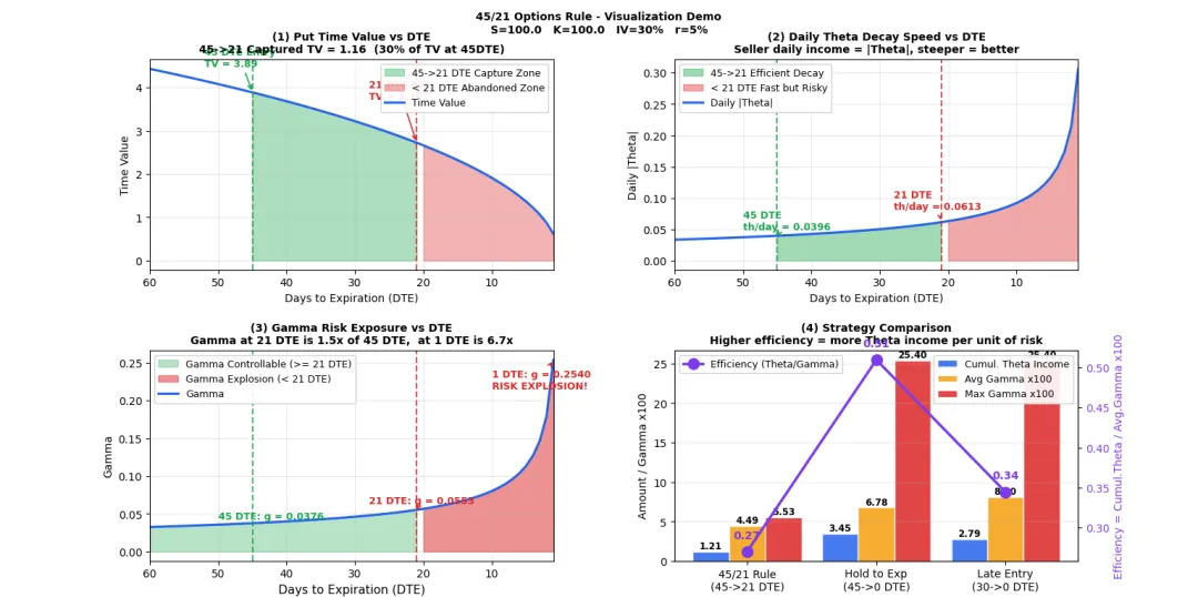
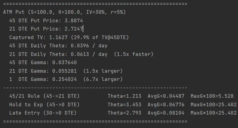
图1（左上）时间价值那张图呈现的是一条从左上向右下递减的曲线。在45天时，这张期权的时间价值约为3.89；到21天时还剩2.72。这24天的持仓期内，卖方捕获了1.16的时间价值，约占45天时刻全部可用时间价值的30%。乍看之下这个数字不算高，但这正是45/21法则保守收割的代价——你主动放弃了一部分潜在收入，换来的是远离了到期日前最危险的那段区间。

图2（右上）每日Theta图展示了时间衰减的速度。在45天时，期权每天大约流失0.040的价值；到21天时这个数字上升到0.061，加速了约1.5倍。图中绿色区域是45到21天之间的高效衰减带，红色区域是21天以内的极速衰减带。红色区域虽然每天的Theta绝对值更大（意味着卖方每天理论上赚得更多），但这片区域的实际可操作性非常差，原因在第三张图里一目了然。

图3（左下）Gamma图是整个演示中最具冲击力的一张。在45天时Gamma仅为0.038，意味着标的价格每变动1元，期权Delta只会变化0.038，头寸的调整是温和、可控的。到21天时Gamma升到0.055，是45天的1.5倍，尚在可接受范围内。但到了仅剩1天时，Gamma飙升到0.254，这是45天时的6.7倍。在这个水平上，标的价格哪怕只跳动几分钱，你的Delta就会剧烈摆动，头寸可能在几分钟内从盈利变成巨亏。这就是45/21法则选择在21天离场的核心依据：不是因为你不想多赚那几天的Theta，而是因为继续待下去的Gamma风险已经和收益完全不成比例。

图4（右下）把三种不同策略放在一起做了横向对比。第一种是标准的45/21法则，45天进、21天出，累计Theta收入为1.21，期间平均Gamma仅0.045，最大Gamma也只有0.055。第二种是45天进场但死扛到期的策略，累计Theta确实高得多，达到3.45，但平均Gamma翻了一倍多到0.068，最大Gamma更是飙升到0.254，为了多赚2.24的Theta收入，你需要承受将近5倍的极端风险暴露。第三种是30天晚进场、持有到期的策略，Theta收入2.79，但平均和最大Gamma同样很高，属于两头不靠，既没有享受到45天开仓时的充裕安全边际，也没有在21天及时离场规避尾部风险。

紫色折线标注的效率比（累计Theta除以平均Gamma）是衡量风险调整后收益的核心指标。45/21法则的效率比在三者中遥遥领先，说明它用最低的单位风险换回了最合理的时间价值收入。死扛到期和晚进场策略的效率比都明显偏低，本质上是在用不成比例的高风险去换取边际收益。这就是45/21法则的核心价值所在：它不追求单笔利润最大化，而是追求在可承受的风险范围内，以最高的效率持续、重复地捕获时间价值。

在期权世界里，最昂贵的成本从来不是权利金，而是贪婪。45/21法则教给你的不是如何赚得最多，而是如何在市场这个充满不确定性的赌场里，活得最久、走得最稳。

import numpy as npimport matplotlib.pyplot as pltfrom scipy.stats import normdef d1_calc(S, K, tau, r, q, sigma):return (np.log(S / K) +            (r - q + 0.5 * sigma ** 2) * tau) / (sigma * np.sqrt(tau))def option_price(cp, S, K, tau, r, q, sigma):    d1 = d1_calc(S, K, tau, r, q, sigma)    d2 = d1 - sigma * np.sqrt(tau)if cp == 1:return np.exp(            -q * tau) * S * norm.cdf(d1) \               - np.exp(-r * tau) * K * norm.cdf(d2)else:return -np.exp(            -q * tau) * S * norm.cdf(-d1) \               + np.exp(-r * tau) * K * norm.cdf(-d2)def option_theta_daily(cp, S, K, tau, r, q, sigma):    d1 = d1_calc(S, K, tau, r, q, sigma)    d2 = d1 - sigma * np.sqrt(tau)if cp == 1:        theta_annual = (-np.exp(-q * tau) * (S * norm.pdf(d1) * sigma)                        / (2 * np.sqrt(tau))            + q * np.exp(-q * tau) * S * norm.cdf(d1)            - r * K * np.exp(-r * tau) * norm.cdf(d2)        )else:        theta_annual = (-np.exp(-q * tau) * (S * norm.pdf(d1) * sigma)                        / (2 * np.sqrt(tau))            - q * np.exp(-q * tau) * S * norm.cdf(-d1)            + r * K * np.exp(-r * tau) * norm.cdf(-d2)        )return theta_annual / 365def option_gamma(S, K, tau, r, q, sigma):    d1 = d1_calc(S, K, tau, r, q, sigma)return np.exp(-q * tau) * norm.pdf(d1) / (S * sigma * np.sqrt(tau))S = 100.0K = 100.0r = 0.05q = 0.00sigma = 0.30dte_array = np.arange(60, 0, -1)tau_array = dte_array / 365.0put_price = option_price(-1, S, K, tau_array, r, q, sigma)theta_day = option_theta_daily(-1, S, K, tau_array, r, q, sigma)gamma_vals = option_gamma(S, K, tau_array, r, q, sigma)intrinsic = max(K - S, 0)time_value = put_price - intrinsicdef cum_theta(dte_start, dte_end):    mask = (dte_array <= dte_start) & (dte_array >= dte_end)return np.sum(np.abs(theta_day[mask]))def avg_gamma(dte_start, dte_end):    mask = (dte_array <= dte_start) & (dte_array >= dte_end)return np.mean(gamma_vals[mask])def max_gamma(dte_start, dte_end):    mask = (dte_array <= dte_start) & (dte_array >= dte_end)return np.max(gamma_vals[mask])strategies = {'45/21 Rule\n(45->21 DTE)': (45, 21),'Hold to Exp\n(45->0 DTE)': (45, 1),'Late Entry\n(30->0 DTE)':  (30, 1),}strat_names= list(strategies.keys())strat_theta= []strat_gamma_avg = []strat_gamma_max = []for name, (s, e) in strategies.items():    strat_theta.append(cum_theta(s, e))    strat_gamma_avg.append(avg_gamma(s, e))    strat_gamma_max.append(max_gamma(s, e))fig, axes = plt.subplots(2, 2, figsize=(16, 11))fig.suptitle('45/21 Options Rule - Visualization Demo\n'    f'S={S}   K={K}   IV={sigma:.0%}   r={r:.0%}',fontsize=10, fontweight='bold', y=0.98)fig.subplots_adjust(hspace=0.38, wspace=0.30, top=0.90, bottom=0.06)# Color paletteC_MAIN= '#2563EB'C_ENTRY= '#16A34A'C_EXIT= '#DC2626'# Time Valueax1 = axes[0, 0]ax1.fill_between(dte_array, 0, time_value,where=(dte_array <= 45) & (dte_array >= 21),alpha=0.35, color=C_ENTRY, label='45->21 DTE Capture Zone')ax1.fill_between(dte_array, 0, time_value,where=(dte_array < 21),alpha=0.35, color=C_EXIT, label='< 21 DTE Abandoned Zone')ax1.plot(dte_array, time_value, color=C_MAIN,linewidth=2.2, label='Time Value')ax1.axvline(45, color=C_ENTRY, linestyle='--', linewidth=1.5, alpha=0.8)ax1.axvline(21, color=C_EXIT,  linestyle='--', linewidth=1.5, alpha=0.8)tv_45 = time_value[dte_array == 45][0]tv_21 = time_value[dte_array == 21][0]ax1.annotate(f'45 DTE Entry\nTV = {tv_45:.2f}',xy=(45, tv_45), xytext=(52, tv_45 + 0.6),fontsize=9, color=C_ENTRY, fontweight='bold',arrowprops=dict(arrowstyle='->', color=C_ENTRY, lw=1.2))ax1.annotate(f'21 DTE Exit\nTV = {tv_21:.2f}',xy=(21, tv_21), xytext=(28, tv_21 + 1.0),fontsize=9, color=C_EXIT, fontweight='bold',arrowprops=dict(arrowstyle='->', color=C_EXIT, lw=1.2))captured = tv_45 - tv_21ax1.set_title(f'(1) Put Time Value vs DTE'              f'\n' f'45->21 Captured TV = {captured:.2f}  '              f'({captured/tv_45*100:.0f}% of TV at 45DTE)',fontsize=10, fontweight='bold')ax1.set_xlabel('Days to Expiration (DTE)', fontsize=10)ax1.set_ylabel('Time Value', fontsize=10)ax1.legend(loc='upper right', fontsize=9, framealpha=0.9)ax1.set_xlim(60, 1)ax1.grid(True, alpha=0.3)# Daily Thetaax2 = axes[0, 1]theta_abs = np.abs(theta_day)ax2.fill_between(dte_array, 0, theta_abs,where=(dte_array <= 45) & (dte_array >= 21),alpha=0.40, color=C_ENTRY, label='45->21 Efficient Decay')ax2.fill_between(dte_array, 0, theta_abs,where=(dte_array < 21),alpha=0.40, color=C_EXIT, label='< 21 DTE Fast but Risky')ax2.plot(dte_array, theta_abs, color=C_MAIN,linewidth=2.2, label='Daily |Theta|')ax2.axvline(45, color=C_ENTRY, linestyle='--', linewidth=1.5, alpha=0.8)ax2.axvline(21, color=C_EXIT,  linestyle='--', linewidth=1.5, alpha=0.8)theta_45 = theta_abs[dte_array == 45][0]theta_21 = theta_abs[dte_array == 21][0]ax2.annotate(f'45 DTE\nth/day = {theta_45:.4f}',xy=(45, theta_45), xytext=(50, theta_45 + 0.01),fontsize=9, color=C_ENTRY, fontweight='bold',arrowprops=dict(arrowstyle='->', color=C_ENTRY, lw=1.2))ax2.annotate(f'21 DTE\nth/day = {theta_21:.4f}',xy=(21, theta_21), xytext=(28, theta_21 + 0.02),fontsize=9, color=C_EXIT, fontweight='bold',arrowprops=dict(arrowstyle='->', color=C_EXIT, lw=1.2))ax2.set_title('(2) Daily Theta Decay Speed vs DTE\n'              'Seller daily income = |Theta|, steeper = better',fontsize=10, fontweight='bold')ax2.set_xlabel('Days to Expiration (DTE)', fontsize=10)ax2.set_ylabel('Daily |Theta|', fontsize=10)ax2.legend(loc='upper left', fontsize=9, framealpha=0.9)ax2.set_xlim(60, 1)ax2.grid(True, alpha=0.3)# Gammaax3 = axes[1, 0]ax3.fill_between(dte_array, 0, gamma_vals,where=(dte_array >= 21),alpha=0.30, color=C_ENTRY, label='Gamma Controllable (>= 21 DTE)')ax3.fill_between(dte_array, 0, gamma_vals,where=(dte_array < 21),alpha=0.50, color=C_EXIT, label='Gamma Explosion (< 21 DTE)')ax3.plot(dte_array, gamma_vals, color=C_MAIN, linewidth=2.2, label='Gamma')ax3.axvline(45, color=C_ENTRY, linestyle='--', linewidth=1.5, alpha=0.8)ax3.axvline(21, color=C_EXIT,  linestyle='--', linewidth=1.5, alpha=0.8)gamma_45 = gamma_vals[dte_array == 45][0]gamma_21 = gamma_vals[dte_array == 21][0]gamma_1  = gamma_vals[dte_array == 1][0]ax3.annotate(f'45 DTE: g = {gamma_45:.4f}',xy=(45, gamma_45), xytext=(50, gamma_45 + 0.005),fontsize=9, color=C_ENTRY, fontweight='bold')ax3.annotate(f'21 DTE: g = {gamma_21:.4f}',xy=(21, gamma_21), xytext=(28, gamma_21 + 0.008),fontsize=9, color=C_EXIT, fontweight='bold',arrowprops=dict(arrowstyle='->', color=C_EXIT, lw=1.2))ax3.annotate(f'1 DTE: g = {gamma_1:.4f}\nRISK EXPLOSION!',xy=(1, gamma_1), xytext=(10, gamma_1 * 0.85),fontsize=9, color=C_EXIT, fontweight='bold',arrowprops=dict(arrowstyle='->', color=C_EXIT, lw=1.2))ax3.set_title(f'(3) Gamma Risk Exposure vs DTE'              f'\n'f'Gamma at 21 DTE is '              f'{gamma_21/gamma_45:.1f}x of 45 DTE, '              f'at 1 DTE is {gamma_1/gamma_45:.1f}x',fontsize=10, fontweight='bold')ax3.set_xlabel('Days to Expiration (DTE)', fontsize=11)ax3.set_ylabel('Gamma', fontsize=10)ax3.legend(loc='upper left', fontsize=9, framealpha=0.9)ax3.set_xlim(60, 1)ax3.grid(True, alpha=0.3)# Strategy Comparisonax4 = axes[1, 1]x_pos = np.arange(len(strat_names))bar_w = 0.28bars1 = ax4.bar(x_pos - bar_w, strat_theta, bar_w,color=C_MAIN, alpha=0.85, label='Cumul. Theta Income', edgecolor='white')bars2 = ax4.bar(x_pos, [g * 100 for g in strat_gamma_avg], bar_w,color='#F59E0B', alpha=0.85, label='Avg Gamma x100', edgecolor='white')bars3 = ax4.bar(x_pos + bar_w, [g * 100 for g in strat_gamma_max], bar_w,color=C_EXIT, alpha=0.85, label='Max Gamma x100', edgecolor='white')for bars in [bars1, bars2, bars3]:for bar in bars:        h = bar.get_height()        ax4.text(bar.get_x() + bar.get_width() / 2, h + 0.02,f'{h:.2f}', ha='center', va='bottom', fontsize=8.5, fontweight='bold')ax4_twin = ax4.twinx()efficiency = [t / (g * 100) if g > 0else 0 for t, g in zip(strat_theta, strat_gamma_avg)]ax4_twin.plot(x_pos, efficiency, 'o-', color='#7C3AED', linewidth=2.5,markersize=10, label='Efficiency (Theta/Gamma)', zorder=5)for i, eff in enumerate(efficiency):    ax4_twin.annotate(f'{eff:.2f}', xy=(i, eff), xytext=(0, 12),textcoords='offset points', fontsize=10, fontweight='bold',color='#7C3AED', ha='center')ax4_twin.set_ylabel('Efficiency = Cumul.Theta / Avg.Gamma x100',fontsize=10, color='#7C3AED')ax4_twin.tick_params(axis='y', labelcolor='#7C3AED')ax4.set_title('(4) Strategy Comparison\n'              'Higher efficiency = more Theta income per unit of risk',fontsize=10, fontweight='bold')ax4.set_xticks(x_pos)ax4.set_xticklabels(strat_names, fontsize=10)ax4.set_ylabel('Amount / Gamma x100', fontsize=10)ax4.legend(loc='upper right', fontsize=9, framealpha=0.9)ax4_twin.legend(loc='upper left', fontsize=9, framealpha=0.9)ax4.grid(True, alpha=0.3, axis='y')plt.show()print('=' * 60)print(f'ATM Put (S={S}, K={K}, IV={sigma:.0%}, r={r:.0%})')print(f'  45 DTE Put Price: {put_price[dte_array==45][0]:.4f}')print(f'  21 DTE Put Price: {put_price[dte_array==21][0]:.4f}')print(f'  Captured TV: {captured:.4f} ({captured/tv_45*100:.1f}% of TV@45DTE)')print(f'  45 DTE Daily Theta: {theta_45:.4f} / day')print(f'  21 DTE Daily Theta: {theta_21:.4f} / day  '      f'({theta_21/theta_45:.1f}x faster)')print(f'  45 DTE Gamma: {gamma_45:.6f}')print(f'  21 DTE Gamma: {gamma_21:.6f}  ({gamma_21/gamma_45:.1f}x larger)')print(f'  1  DTE Gamma: {gamma_1:.6f}  ({gamma_1/gamma_45:.1f}x larger)')print('-' * 60)for name, t, g_a, g_m in zip(        strat_names, strat_theta, strat_gamma_avg, strat_gamma_max):    nm = name.replace('\n', ' ')print(f'  {nm:30s}  Theta={t:.3f}  AvgG={g_a:.5f}  MaxG*100={g_m*100:.3f}')print('=' * 60)