Python绘制主成分/因子分析+相关性分析组合图
- 2026-10-11 06:14:48
Python绘制主成分/因子分析+相关性分析组合图

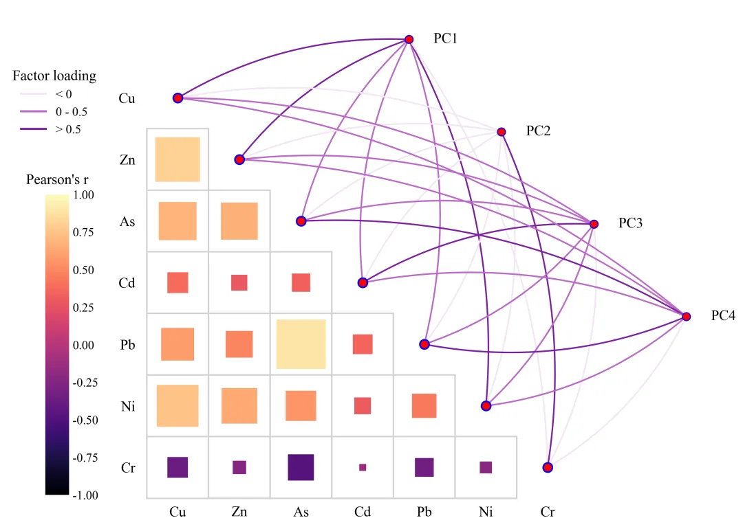
这张图的左下部分是一个相关性矩阵,通过方块的颜色和大小来展示两两特征之间的皮尔逊相关性,方块越大表示相关性越强。图的上半部分是因子分析或主成分分析的可视化,对角线上的红点代表各个特征,右侧的红点代表提取的主成分;连接特征与主成分的弧线颜色代表因子载荷的强度。 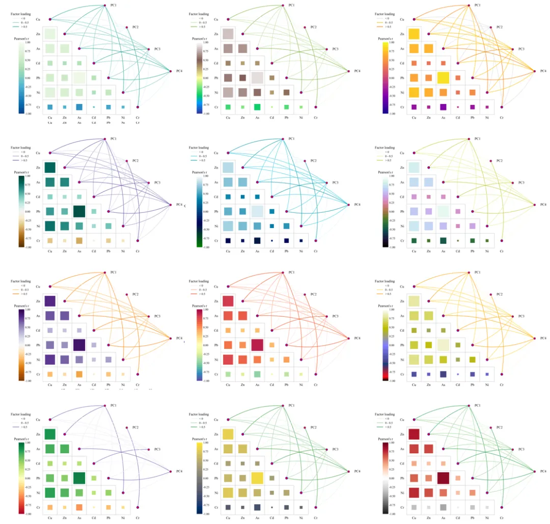
多种配色 



库的导入以及字体设置 

颜色库设置以及配色方案的选择 

绘图函数 

数据的加载以及预处理 

主成分分析/因子分析 

绘图 

2.设置主成分的数量: 3.设置绘图结果的保存地址: 4.设置原始数据的输入路径: 

期刊图片复现|Python绘制二维偏依赖PDP图 期刊复现|python绘制基于SHAP分析和GAM模型拟合的单特征依赖图 期刊图片复现|python绘制带有渐变颜色shap特征重要性组合图(条形图+蜂巢图) 期刊复现|用Python绘制SHAP特征重要性总览图、依赖图、双特征交互效应SHAP图,解锁XGBoost模型的终极奥秘 期刊图片复现|Python绘制shap重要性蜂巢图+单特征依赖图+交互效应强度气泡图+交互效应依赖图(回归+二分类+分类) 

需要的请后台私信我获取详细信息,注意只会分享练习数据和代码文件,不会提供答疑服务,代码文件中已经包含了每行代码的完整注释!!!
代码绘制成果展示
代码解释
第一部分
# =========================================================================================# ====================================== 1. 库的导入 =========================================# =========================================================================================import matplotlibimport pandas as pdimport numpy as npimport matplotlib.pyplot as pltfrom sklearn.preprocessing import StandardScalerfrom sklearn.decomposition import PCAimport matplotlib.patches as patchesfrom matplotlib.colors import Normalizeimport matplotlib.colorbar as colorbarfrom matplotlib.lines import Line2Dfrom factor_analyzer import FactorAnalyzermatplotlib.rcParams['pdf.fonttype'] = 42matplotlib.rcParams['ps.fonttype'] = 42plt.rcParams['font.family'] = 'serif'plt.rcParams['font.serif'] = ['Times New Roman']plt.rcParams['axes.unicode_minus'] = Falseplt.rcParams['mathtext.fontset'] = 'stix'
第二部分
# =========================================================================================# ====================================== 2.颜色库 =========================================# =========================================================================================COLOR_SCHEMES = {1: {'neg_loading': '#D3D3D3', 'weak_pos_loading': '#B0C4DE', 'strong_pos_loading': '#F08080','corr_cmap': 'RdBu_r'},}SELECTED_SCHEME = 20#配色方案N_COMPONENTS = 4 # 设置主成分分析(PCA)要提取的主成分数量
第三部分
接收相关矩阵、载荷、特征名称、配色方案ID和主成分数量作为参数
# =========================================================================================# ====================================== 3. 绘图函数 =========================================# =========================================================================================def plot_correlation_and_pca(corr_matrix, loadings, metals, scheme_id,n_components): # 定义主绘图函数...n_features = len(metals) # 获取特征的数量scheme = COLOR_SCHEMES.get(scheme_id, COLOR_SCHEMES[1]) # ...获取配色方案fig, ax = plt.subplots(figsize=(16, 9), facecolor='white')COLOR_NEG_LOADING = scheme['neg_loading'] # ...COLOR_WEAK_POS_LOADING = scheme['weak_pos_loading'] # ...COLOR_STRONG_POS_LOADING = scheme['strong_pos_loading'] # ...corr_cmap = plt.get_cmap(scheme['corr_cmap']) # ...corr_norm = Normalize(vmin=-1, vmax=1) # 归一化,将-1到1的相关系数映射到0-1的颜色范围grid_line_width = 1.5 # ...grid_line_color = 'lightgray' # ...z_order = 1.5 # ...# ... [绘制网格线] ...for i in range(1, n_features): # 循环绘制从第1条到倒数第2条的水平线ax.plot([0, i], [i, i], color=grid_line_color, linewidth=grid_line_width, zorder=z_order)for j in range(1, n_features): # 循环绘制从第1条到倒数第2条的垂直线ax.plot([j, j], [j, n_features], color=grid_line_color, linewidth=grid_line_width, zorder=z_order)# 填充背景色块和数据色块for i in range(n_features): # ...for j in range(n_features): # ...if i >= j: # 主对角线及其左下方区域rect_bg = patches.Rectangle((j, i), 1, 1, facecolor='white', edgecolor='none', zorder=1)ax.add_patch(rect_bg)if i > j: # 主对角线以下的区域 (相关性矩阵)x, y = j + 0.5, i + 0.5 # ...corr_val = corr_matrix.iloc[i, j] # ...size = abs(corr_val) * 0.9 # 方块大小由相关性绝对值决定color = corr_cmap(corr_norm(corr_val)) # 方块颜色由相关性值决定# ...rect_fg = patches.Rectangle((bottom_left_x, bottom_left_y), size, size,linewidth=1.5, edgecolor='none',facecolor=color, zorder=2)ax.add_patch(rect_fg)ax.set_xticks(np.arange(n_features) + 0.5) # ...ax.set_xticklabels(metals, fontsize=14) # ...ax.set_yticks(np.arange(n_features) + 0.5) # ...ax.set_yticklabels(metals, fontsize=14) # ...ax.tick_params(axis='x', bottom=True, top=False, labelbottom=True, labeltop=False, pad=-15)ax.tick_params(axis='y', left=True, right=False, labelleft=True, labelright=False, pad=-15)ax.invert_yaxis() # 翻转y轴,使(0,0)在左上角# ==================== 绘制PCA载荷连接 ====================metal_node_coords = [(i + 0.5, i + 0.5) for i in range(n_features)] # 变量节点(在对角线上)# ... [计算PC(因子)节点的位置] ...pc_center_x = n_features - 0.5pc_center_y = n_features / 2 - 1.7spread_per_node = 1.5# ...offsets = np.linspace(start_offset, end_offset, n_components)# ... [创建图例] ...legend_elements = [Line2D([0], [0], color=COLOR_NEG_LOADING, lw=2, label='< 0'),Line2D([0], [0], color=COLOR_WEAK_POS_LOADING, lw=2, label='0 - 0.5'),Line2D([0], [0], color=COLOR_STRONG_POS_LOADING, lw=2, label='> 0.5')]ax.legend(handles=legend_elements, title='Factor loading',loc='upper left', bbox_to_anchor=(-0.2, 0.9),fontsize=12, title_fontsize=14, frameon=False)# ... [创建颜色条 Colorbar] ...cbar_ax = fig.add_axes([0.2, 0.15, 0.02, 0.45]) # [左, 下, 宽, 高]cb = colorbar.ColorbarBase(cbar_ax, cmap=corr_cmap, norm=corr_norm, orientation='vertical')cb.outline.set_visible(False)cb.ax.tick_params(length=0)cb.ax.set_title("Pearson's r", size=14, pad=10)cb.ax.yaxis.set_ticks_position('right')cb.ax.tick_params(labelsize=12)ax.spines[['top', 'right', 'left', 'bottom']].set_visible(False) # 隐藏所有坐标轴ax.tick_params(axis='both', which='both', length=0) # 隐藏刻度ax.set_aspect('equal', adjustable='box') # 保持宽高比为1plt.savefig(output_filename_png, dpi=300, bbox_inches='tight', facecolor='white')plt.savefig(output_filename_pdf, bbox_inches='tight', facecolor='white')plt.close(fig)print(f"绘图成功!结果已保存为 '{output_filename_png}' 和 '{output_filename_pdf}'")
第四部分
# =========================================================================================# ======================================4.数据的加载及预处理=========================================# =========================================================================================# ==================== 1. 从本地Excel文件加载数据 ====================excel_path = r'data.xlsx' # 数据文件的路径df = pd.read_excel(excel_path) #读取数据print(f"成功从 '{excel_path}' 加载数据。")metals = df.columns.tolist() # 获取DataFrame的所有列名,并转换为一个列表# ==================== 2. 执行统计分析 ====================corr_matrix = df.corr() # 计算DataFrame中各列之间的皮尔逊相关系数,并生成相关系数矩阵scaler = StandardScaler() # 创建一个StandardScaler对象,用于数据标准化numeric_df = df.select_dtypes(include=np.number) # 从原始DataFrame中选择所有数值类型的列metals = numeric_df.columns.tolist()scaled_data = scaler.fit_transform(numeric_df) # 对数值数据进行拟合和转换,即进行标准化处理
第五部分
初始化 FactorAnalyzer,设置因子数量,使用主成分法来提取因子。使用方差最大化旋转。
# =========================================================================================# ====================================== 6. 主成分分析=========================================# =========================================================================================# pca = PCA(n_components=N_COMPONENTS) # 创建一个PCA对象,并指定要提取的主成分数量# pca.fit(scaled_data) # 使用标准化后的数据来训练PCA模型# loadings = pca.components_.T # 获取PCA的载荷矩阵...#初始化模型# n_factors主成分数量# method='principal'用主成分法#rotation='varimax'用“方差最大化”旋转fa = FactorAnalyzer(n_factors=N_COMPONENTS, method='principal', rotation='varimax')# 训练模型fa.fit(scaled_data)# 获取旋转后的载荷矩阵loadings = fa.loadings_
第六部分
# =========================================================================================# ====================================== 7. 绘图 =========================================# =========================================================================================plot_correlation_and_pca(corr_matrix, loadings, metals, scheme_id=SELECTED_SCHEME, n_components=N_COMPONENTS)
如何应用?
1.选择你想要使用到的配色方案:
SELECTED_SCHEME = 20#配色方案N_COMPONENTS = 4output_filename_png = fr'correlation_pca_{scheme_id}.png'output_filename_pdf = fr'correlation_pca_{scheme_id}.pdf'
excel_path = r'data.xlsx'推荐
获取方式
本文来自网友投稿或网络内容,如有侵犯您的权益请联系我们删除,联系邮箱:596563534@qq.com 。
