期刊方法模仿|Python实现多策略采样驱动的集成机器学习二分类任务解释建模框架
- 2026-06-27 11:41:00
期刊方法模仿|Python实现多策略采样驱动的集成机器学习二分类任务解释建模框架

论文:Towards improved identification of residential land vulnerable to abandonment in rural China: A case study using an integration approach of machine learning techniques 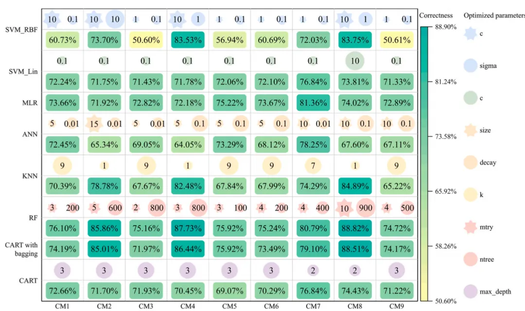
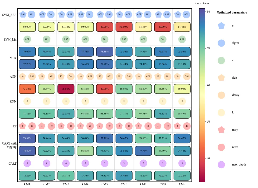
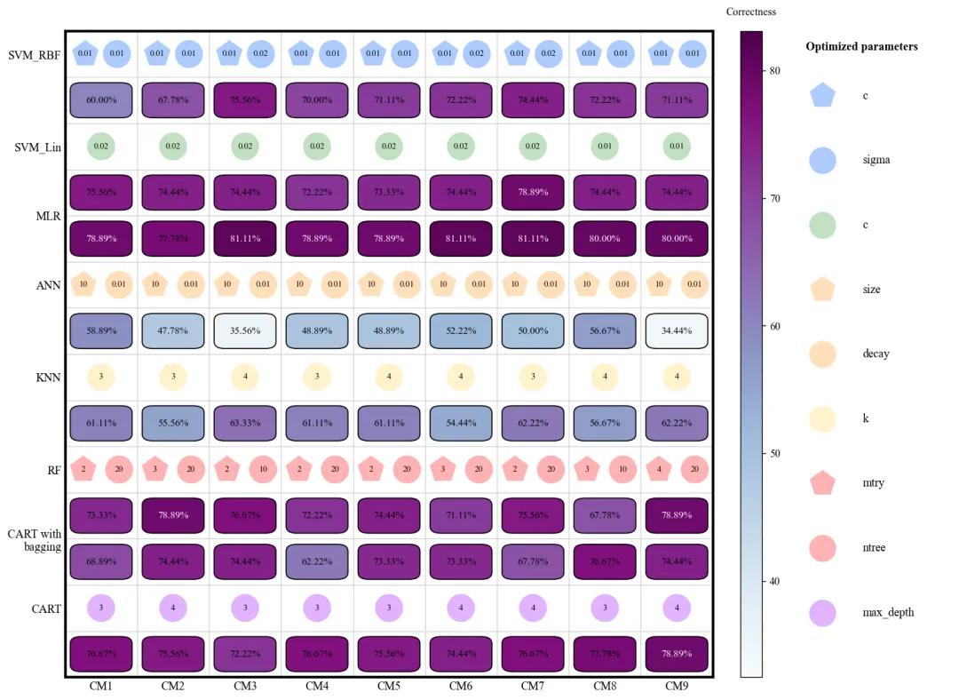
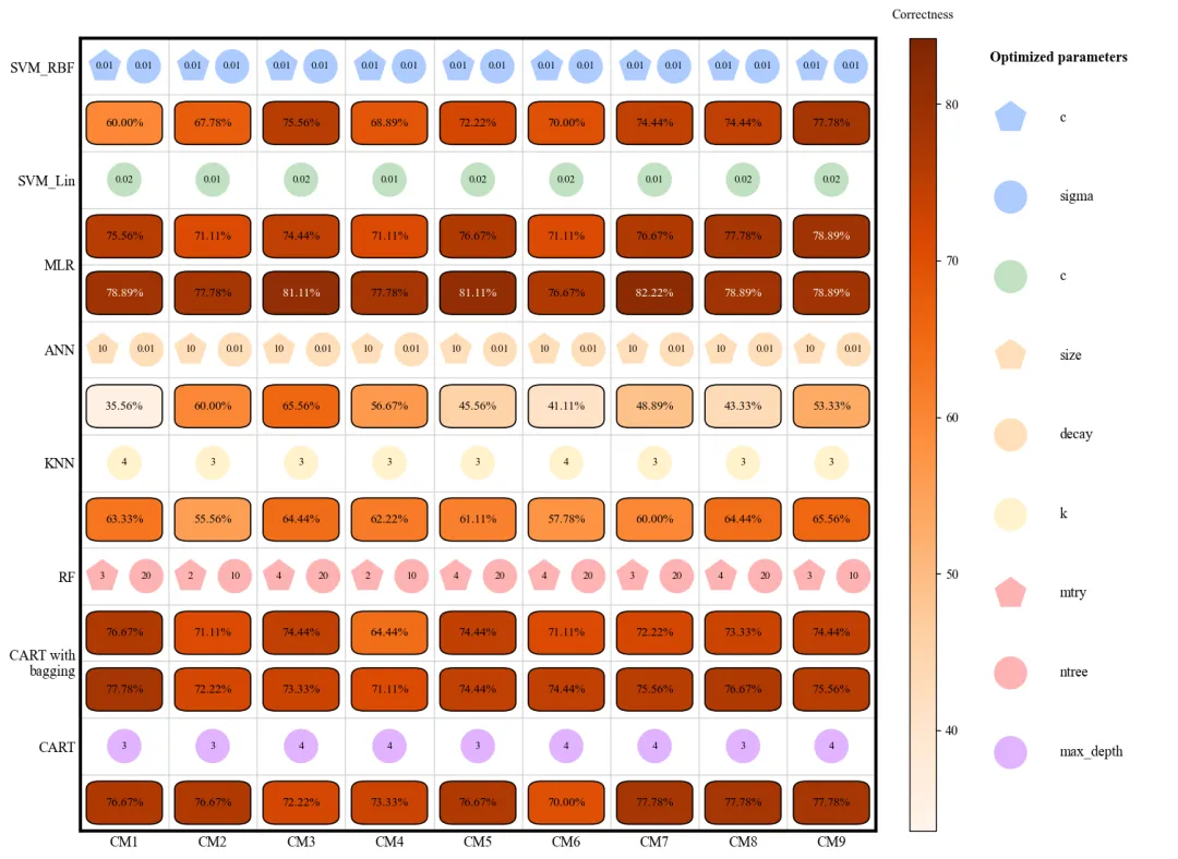
各模型优化的参数值与验证准确率 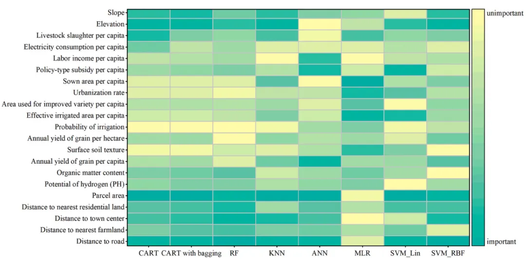
不同模型的特征变量的重要性排序 论文原图 本文通过集成 9 种不同的采样方法(包括原始采样、过采样、欠采样以及基于高程、坡度、NDVI 等地理因子的分层采样)来处理数据类别不平衡问题,并自动配置 8 种机器学习模型进行超参数网格搜索优化;随后利用独立测试集验证模型性能,结合 SHAP 解释性分析各特征的重要性排名,最后通过多模型硬投票机制对数据进行预测,输出模型准确率对比图、特征重要性热力图及最终集成预测结果。 注意,此为我对原文方法的拙劣模仿,并非完全还原原文方法,可能存在不足之处,使用时还请仔细阅读原文后进行修改再行应用 
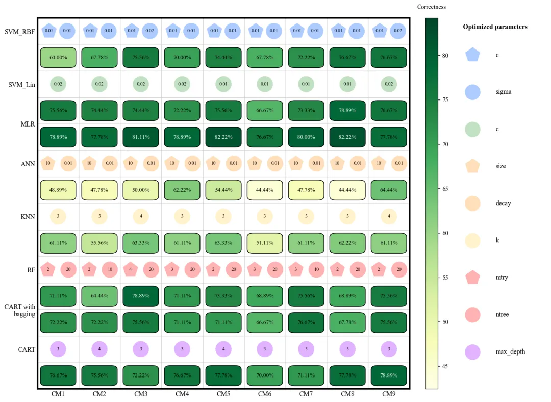
此图展示了 8 种机器学习模型在 9 种不同采样方法(CM1-CM9)下的验证准确率及其对应的最优超参数配置。图中纵轴代表不同的模型算法,横轴代表不同的采样策略,深蓝色方框表示较高的准确率,而浅黄色或绿色则表示性能较低。每个模型上方的小图标直观地标注了经过网格搜索优化后的超参数参数值(如 SVM 的惩罚因子、KNN 的近邻数 以及随机森林的决策树数量 等)。从整体趋势来看,MLR、RF、CART with bagging以及CART在多种采样环境下表现出较强的稳健性,准确率普遍维持在 70%-78% 左右;相比之下,SVM_RBF和ANN的性能波动较大,这表明这两个模型对样本均衡策略的选择更为敏感。 
此图揭示了各评价因子对预测结果的影响权重,可以清晰地看出elevation和slope在绝大多数模型中均处于深蓝色区域,被公认为最关键的触发因子,而lithology和land_use的重要性排名相对较低,呈现较浅的色调。 仿图 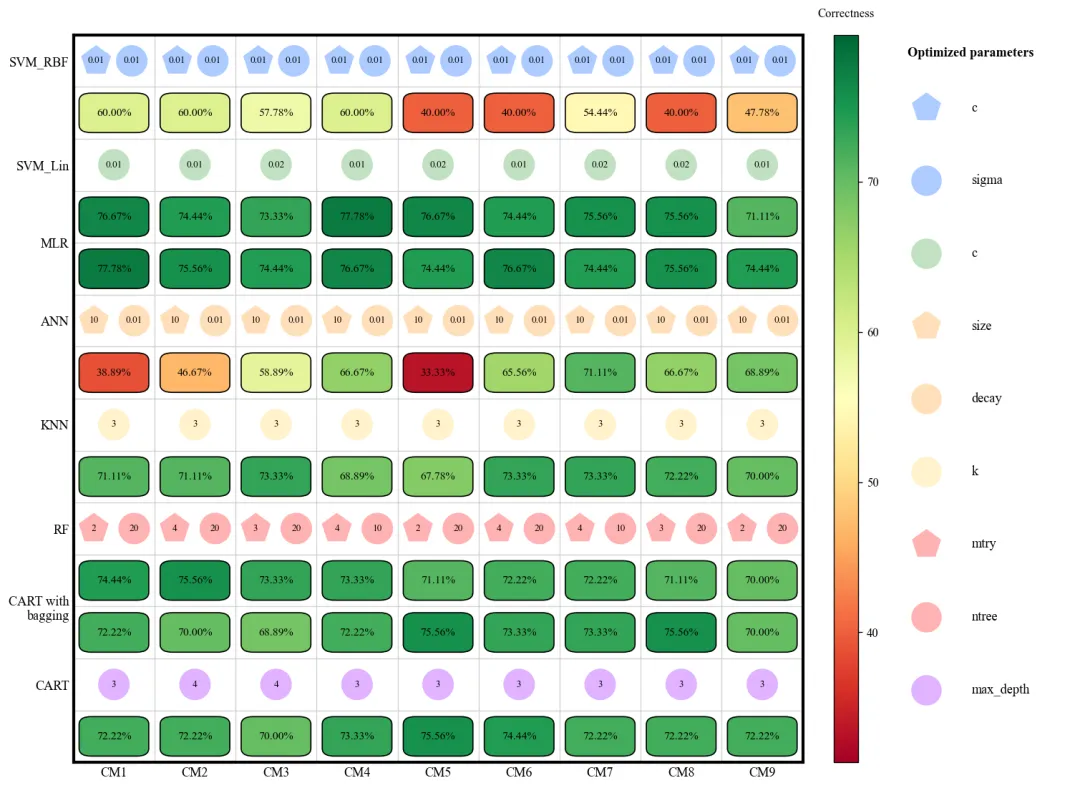
多种配色 


库的导入以及字体设置 

颜色库的设置以及配色方案的选择 

模型性能对比图绘制函数:它根据输入的模型列表动态计算绘图所需的行数,如果模型有超参数,它会分配两行(一行参数,一行准确率);如果没有,则只画一行。分为三部分:主图、颜色条、侧边图例。 颜色深度由准确率决定,并自动根据背景深浅切换文字颜色。绘制不同形状的图标,表示不同超参数指标,并在图标中心标注该采样方法下的最优参数值。 

多模型重要性对比热图绘制函数:此函数绘制特征重要性排名热图。首先对特征进行重新排序,计算每个特征在所有模型中的排名总和,总和越小的排在前面(代表综合重要性最高)。通过颜色条显示两个极端标签(最高排名和最低排名),直观地解释哪些特征是影响预测的关键因子。 

重要性计算辅助函数:模型解释的核心。使用SHAP来评估特征重要性。为了加快计算速度,进行了背景数据采样。根据模型类型选择最高效的解释器。树模型用 

采样辅助函数:在实际任务中,负类样本往往远多于正类样本。函数将负样本分成多个箱子。从每个箱子中抽取相同数量的样本,确保采得的负样本在分布上是均匀且具有代表性的。最后通过随机补漏或多余剔除,确保最终得到的样本数严格等于目标数量。 

执行部分:首先指定了存放数据的本地路径和结果的保存路径,随后加载的Excel 数据。定义了 9 种采样实验方法和 8 种机器学习模型。定义空矩阵,准备用来记录每个模型在每种采样方法下的准确率得分。 

执行部分:模型参数配置与数据分割,列出了8个模型及其对应的参数搜索范围。将数据切分训练和测试集。对特征进行归一化,确保不同量级的特征在模型中具有平等的权重。最后将数据还原为带列名的DataFrame方便后续分析。 

执行部分:采样方法循环逻辑。CM1:原始数据。CM2:过采样。CM3:欠采样。CM4:正负样本都往中间靠拢,混合重采样。CM5-9:按地理因子采样。 CM5按每 300 米海拔划分区域抽取负类,CM6 按坡度,CM7 按土地类型。 

执行部分:模型训练与保存最优模型,对当前数据集下的每个模型执行网格搜索。尝试不同的参数组合,通过 5 折交叉验证选出最强组合。计算最强模型在独立测试集上的准确率。会进行 9 种采样方法比对,帮每个模型保留它在所有实验中表现最好的那一次。这些最佳模型将用于最后的 SHAP 解释和集成预测。 

执行部分:绘制准确率与参数对比图,把各个模型在 9 种方法下找出的参数值一个个提取出来,并赋予它们特定的形状颜色。最后,调用之前定义的函数进行绘图。 

执行部分:特征重要性热图,取出 8 个最强模型,对每一个模型调用重要性辅助函数,计算shap值。算完后,所有特征在不同模型里的排名会被合并。最后绘制成图。 

执行部分:最终集成预测,将全部数据按照之前的标准进行标准化。让 8 个最强模型都对数据进行预测。使用投票逻辑,如果 8 个模型里有 5 个或更多认为某点是正类,那最终预测就是正类。将所有中间预测结果和最终投票结果保存成一个文件,打印总准确率。 


期刊图片复现|Python绘制二维偏依赖PDP图 期刊复现|python绘制基于SHAP分析和GAM模型拟合的单特征依赖图 期刊图片复现|python绘制带有渐变颜色shap特征重要性组合图(条形图+蜂巢图) 期刊复现|用Python绘制SHAP特征重要性总览图、依赖图、双特征交互效应SHAP图,解锁XGBoost模型的终极奥秘 期刊图片复现|Python绘制shap重要性蜂巢图+单特征依赖图+交互效应强度气泡图+交互效应依赖图(回归+二分类+分类) 

公众号中的所有所有的免费代码都已经下架了,都并入到付费部分里了,付费合集代码和数据的购买通道已经开通,全部合集100元,后续将会持续更新,决定购买请后台私信我,注意只会分享练习数据和代码文件,不会提供答疑服务,代码文件中已经包含了每行代码的完整注释,购买前请确保真的需要!!!
代码绘制成果展示
代码解释
第一部分
import matplotlib.pyplot as pltimport numpy as npimport pandas as pdimport osimport warningsfrom sklearn.linear_model import LogisticRegressionfrom sklearn.neural_network import MLPClassifierfrom sklearn.neighbors import KNeighborsClassifierfrom sklearn.ensemble import RandomForestClassifier, BaggingClassifierfrom sklearn.tree import DecisionTreeClassifierfrom sklearn.utils import resamplefrom tqdm import tqdm
第二部分
COLOR_SCHEMES = {1: {'cmap': 'YlGnBu','shapes': {'SVM_RBF': '#accbff', 'SVM_Lin': '#c1e1c1', 'ANN': '#ffdfba','KNN': '#fff2cc', 'RF': '#ffb3b3', 'CART': '#e0b3ff'}}SCHEME_ID = 16 # 设置使用的颜色方案CURRENT_CONFIG = COLOR_SCHEMES.get(SCHEME_ID, COLOR_SCHEMES[1]) # 获取颜色方案cmap = plt.get_cmap(CURRENT_CONFIG['cmap']) # 主图颜色current_shape_colors = CURRENT_CONFIG['shapes'] # 形状颜色
第三部分
def save_model_performance_heatmap(accuracy_data, models, cm_labels, param_configs, shape_color_dict, output_filename):row_info = [] # 存储行信息的列表label_y_positions = [] # Y轴标签位置的列表current_y = 0 # 初始化当前Y坐标# 遍历每一个模型for i in range(len(models)):start_y = current_y # 记录当前模型的起始Y坐标if i in param_configs: row_info.append(('icon', i)); current_y += 1 # 如果该模型有参数配置,添加一行用于图标显示row_info.append(('box', i)); # 添加一行用于显示准确率的方框# 计算模型名称标签在Y轴的中心位置label_y_positions.append((start_y + current_y - 1) / 2);current_y += 1 # Y坐标total_physical_rows = current_y # 记录总行数# 创建画布fig = plt.figure(figsize=(15, 11), dpi=120)gs = gridspec.GridSpec(1, 3, width_ratios=[12, 0.4, 3], wspace=0.1) # 设置网格布局ax_main, ax_cbar, ax_leg = fig.add_subplot(gs[0]), fig.add_subplot(gs[1]), fig.add_subplot(gs[2]) # 获取三个子图的坐标轴对象ax_main.set_xlim(-0.5, len(cm_labels) - 0.5); # 主图X轴范围ax_main.set_ylim(-0.5, total_physical_rows - 0.5); # 主图Y轴范围ax_main.invert_yaxis() # 反转Y轴norm = plt.Normalize(vmin=accuracy_data.min() - 2, vmax=accuracy_data.max() + 2) # 设置颜色映射的归一化范围# 遍历每一行行进行绘制for physical_y, (content_type, m_idx) in enumerate(row_info):if content_type == 'box': # 如果是准确率行for j in range(len(cm_labels)): # 遍历每列acc = accuracy_data[m_idx, j] # 获取对应的准确率数值# 创建圆角矩形rect = FancyBboxPatch((j - 0.43, physical_y - 0.38), # 左下角坐标0.86, # 宽度0.76, # 高度boxstyle="round,pad=0,rounding_size=0.15", # 样式:圆角,无内边距,圆角半径facecolor=cmap(norm(acc)), # 填充颜色zorder=2) # 绘图层级ax_main.add_patch(rect); # 将矩形添加到图表中# 添加文本ax_main.text(j, # xphysical_y, # yf"{acc:.2f}%", # 文本内容ha='center', # 水平对齐va='center', # 垂直对齐fontsize=9.5, # 字体大小color='white' if acc > 78 else 'black', # 字体颜色zorder=3) # 绘图层级ax_main.set_xticks(np.arange(len(cm_labels))); # X轴刻度位置ax_main.set_xticklabels(cm_labels, fontsize=11) # X轴刻度标签ax_main.set_yticks(label_y_positions); # Y轴刻度位置ax_main.set_yticklabels(models, fontsize=11); # Y轴刻度标签ax_main.tick_params(length=0) # 隐藏刻度线# 绘制颜色条并设置标题fig.colorbar(plt.cm.ScalarMappable(cmap=cmap, norm=norm), cax=ax_cbar).ax.set_title('Correctness', fontsize=10,pad=15)ax_leg.set_axis_off(); # 关闭图例子图的坐标轴显ax_leg.set_xlim(0, 1); # 图例X轴范围ax_leg.set_ylim(-0.5, 9.5); # 图例Y轴范围ax_leg.invert_yaxis() # 反转Y轴
第四部分
def save_variable_importance_heatmap(importance_df, output_filename):importance_df['sum'] = importance_df.sum(axis=1) # 每个变量在所有模型中的排名总和importance_df = importance_df.sort_values(by='sum', ascending=True) # 根据排名总和进行升序排序importance_df = importance_df.drop(columns=['sum']) # 删除辅助列variables = importance_df.index.tolist() # Y轴标签models = importance_df.columns.tolist() # X轴标签data = importance_df.values # 获取数值# 特征总数量num_vars = len(variables)# 创建画布fig, ax = plt.subplots(figsize=(14, 10), dpi=120)# 获取颜色映射discrete_cmap = plt.get_cmap(CURRENT_CONFIG['cmap'], num_vars)ax.set_xticks(np.arange(len(models))) # X轴主刻度的位置ax.set_yticks(np.arange(len(variables))) # Y轴主刻度的位置ax.set_xticklabels(models, fontsize=16) # X轴刻度标签ax.set_yticklabels(variables, fontsize=16) # Y轴刻度标签ax.set_xticks(np.arange(len(models) + 1) - 0.5, minor=True) # X轴次刻度位置ax.set_yticks(np.arange(len(variables) + 1) - 0.5, minor=True) # Y轴次刻度位置# 在次刻度位置绘制网格线ax.grid(which="minor", color="lightgray", linestyle='-', linewidth=1.5)ax.tick_params(which="minor", bottom=False, left=False) # 隐藏次刻度的刻度线ax.tick_params(length=0) # 主刻度的长度# 颜色条刻度的文本标签cbar.set_ticklabels(['Lowest Rank\n(Unimportant)', 'Highest Rank\n(Important)'])
第五部分
TreeExplainer,线性模型用 LinearExplainer,而SVM或神经网络则使用 KernelExplainer。进行了鲁棒性处理,如果特定解释器报错,它会自动回退到通用的 KernelExplainer。获取SHAP值后,取绝对值的平均数作为得分,最后将其转换为排名。def get_feature_importance(model, X_train, X_val, feature_names, model_name):# 注意:X_train 用于构建解释器背景,X_val 用于计算SHAP值background = shap.utils.sample(X_train, 300) # 从训练集中采样背景数据X_eval = shap.utils.sample(X_val, 300) # 从验证集中采样样本用于计算SHAP值if model_name in ['RF', 'CART']: # 树模型explainer = shap.TreeExplainer(model) # 初始化解释器shap_values = explainer.shap_values(X_eval, check_additivity=False) # 计算SHAP值elif model_name in ['MLR']: # 线性模型explainer = shap.LinearExplainer(model, background) # 初始化,传入背景数据shap_values = explainer.shap_values(X_eval) # 计算SHAP值else: # 数组if len(shap_values.shape) == 3: # 样本数 x 特征数 x 类别数vals = shap_values[:, :, 1] # 提取正类else: # 2维数组vals = shap_values # 直接使用该数组importance_values = np.abs(vals).mean(axis=0) # 计算特征重要性importance_series = pd.Series(importance_values, index=feature_names) # 转换为Seriesranks = importance_series.rank(ascending=True, method='first') # 排名return ranks # 返回排名
第六部分
def stratified_sample(non_landslides, bin_col, n_total_target):unique_bins = non_landslides[bin_col].dropna().unique() # 获取分箱列中的唯一值n_bins = len(unique_bins) # 箱子的数量if n_bins == 0: # 如果没有箱子return non_landslides.sample(n=n_total_target, replace=True) # 直接进行有放回随机采样samples_per_bin = n_total_target // n_bins # 每个箱子应采样的数量sampled_dfs = [] # 采样结果# 遍历每个箱子for b in unique_bins:bin_data = non_landslides[non_landslides[bin_col] == b] # 获取当前箱子的数据# 如果箱内有数据if len(bin_data) > 0:replace = len(bin_data) < samples_per_bin # 如果数据量不足,则允许有放回采样sampled_dfs.append(bin_data.sample(n=samples_per_bin, replace=replace)) # 进行采样并添加至列表elif len(result) > n_total_target:result = result.sample(n=n_total_target, replace=False) # 随机抽样至目标量return result # 最终采样结果
第七部分
if __name__ == "__main__":base_path = r"" # 基础路径save_dir = os.path.join(base_path, "modeling_results") # 保存路径# 如果不存在,创建if not os.path.exists(save_dir):os.makedirs(save_dir)# 原始数据raw_data_path = os.path.join(save_dir, "data.xlsx")df_raw = pd.read_excel(raw_data_path) # 读取数据cms = ['CM1', 'CM2', 'CM3', 'CM4', 'CM5', 'CM6', 'CM7', 'CM8', 'CM9'] # 采样方法models_names = ['SVM_RBF', 'SVM_Lin', 'MLR', 'ANN', 'KNN', 'RF', 'CART with\nbagging', 'CART'] # 模型名称acc_matrix = np.zeros((8, 9)) # 准确率矩阵optimized_params_raw = {} # 最优参数
第八部分
# 模型配置列表model_configs = [('SVM_RBF', SVC(kernel='rbf', probability=True), {'C': [0.01, 0.02], 'gamma': [0.01, 0.02]}),('SVM_Lin', SVC(kernel='linear', probability=True), {'C': [0.01, 0.02]}),('MLR', LogisticRegression(max_iter=1000), {}),('ANN', MLPClassifier(max_iter=2000, early_stopping=True), {'hidden_layer_sizes': [(10,)], 'alpha': [0.01]}),('KNN', KNeighborsClassifier(), {'n_neighbors': [3, 4]}),('RF', RandomForestClassifier(), {'max_features': [2, 3, 4], 'n_estimators': [10, 20]}),('CART with\nbagging', BaggingClassifier(DecisionTreeClassifier()), {}),('CART', DecisionTreeClassifier(), {'max_depth': [3, 4]})]# 提取模型名model_keys = [cfg[0] for cfg in model_configs]best_models_cache = {name: (0, None, None, None) for name in model_keys} # 初始化最佳模型# 数据分割X_full = df_raw.drop('label', axis=1)y_full = df_raw['label']# 划分训练集和测试集X_train_global, X_test_global, y_train_global, y_test_global = train_test_split(X_full, y_full, test_size=0.3, stratify=y_full, random_state=0)#标准化scaler = StandardScaler()X_train_scaled = scaler.fit_transform(X_train_global)X_test_scaled = scaler.transform(X_test_global)#转回DataFrameX_train_global = pd.DataFrame(X_train_scaled, columns=X_full.columns, index=X_train_global.index)X_test_global = pd.DataFrame(X_test_scaled, columns=X_full.columns, index=X_test_global.index)# 将标准化后的训练集部分合并df_train_source = pd.concat([X_train_global, y_train_global], axis=1)
第九部分
# 遍历每一种方法for cm_idx, cm_name in enumerate(tqdm(cms, desc="Total Progress")):# 从训练集中提取正类和负类landslides = df_train_source[df_train_source['label'] == 1].copy() # 提取正类non_landslides_pool = df_train_source[df_train_source['label'] == 0].copy() # 提取负类n_pos = len(landslides) # 正类数量(训练集)n_neg_pool = len(non_landslides_pool) # 计算负类数量(训练集)df_cm_train = None # 初始化当前方法的训练集if cm_name == 'CM1':df_cm_train = df_train_source.copy() # 直接使用原始训练数据elif cm_name == 'CM2':# 对正类进行过采样landslides_oversampled = resample(landslides, # 正类replace=True, # 有放回采样n_samples=n_neg_pool, # 目标数量,使正负样本数量达到平衡random_state=0) # 随机种子# 合并数据df_cm_train = pd.concat([landslides_oversampled, non_landslides_pool])elif cm_name == 'CM3':# 对负类进行欠采样non_landslides_undersampled = resample(non_landslides_pool,replace=False,n_samples=n_pos,random_state=0)# 合并数据df_cm_train = pd.concat([landslides, non_landslides_undersampled])else:temp_pool = non_landslides_pool.copy() # 复制负类if cm_name == 'CM5':min_elev = temp_pool['elevation'].min() # 最低高程max_elev = temp_pool['elevation'].max() # 最高高程bins = np.arange(np.floor(min_elev), np.ceil(max_elev) + 300, 300) # 分箱区间temp_pool['stratify_bin'] = pd.cut(temp_pool['elevation'], bins=bins, labels=False) # 进行分箱neg_sampled = stratified_sample(temp_pool, 'stratify_bin', n_pos) # 执行分层采样
第十部分
# -------------------------------------------------------------# 模型训练与评估# -------------------------------------------------------------cols_to_drop = [c for c in ['stratify_bin'] if c in df_cm_train.columns] # 需要删除的列df_cm_train = df_cm_train.drop(columns=cols_to_drop).dropna() # 删除列并去除空值df_cm_train = df_cm_train.sample(frac=1, random_state=0).reset_index(drop=True) # 打乱数据# 使用采样后的数据作为训练集X_train = df_cm_train.drop('label', axis=1) # 提取特征y_train = df_cm_train['label'] # 提取标签detailed_results = [] # 初始化结果列表# 遍历每个模型配置for m_idx, (m_name, model, grid) in enumerate(tqdm(model_configs, desc=f"Modeling {cm_name}", leave=False)):if grid: # 如果有参数网格# 初始化网格搜索search = GridSearchCV(model, grid, cv=5, scoring='accuracy', n_jobs=-1)search.fit(X_train, y_train) # 训练和搜索best_model = search.best_estimator_ # 最佳模型best_params = search.best_params_ # 最佳参数else: # 如果没有参数网格best_model = model.fit(X_train, y_train) # 直接训练模型best_params = {} # 参数为空# 使用全局测试集进行评估acc = accuracy_score(y_test_global, best_model.predict(X_test_global)) * 100 # 计算测试集准确率acc_matrix[m_idx, cm_idx] = acc # 将准确率存入矩阵optimized_params_raw[(m_idx, cm_idx)] = best_params # 存储该轮的最优参数# 如果当前模型准确率高于缓存中的历史最高值if acc > best_models_cache[m_name][0]:# 缓存时保存全局测试集,确保SHAP计算使用正确的数据best_models_cache[m_name] = (acc, best_model, X_test_global, y_test_global, X_train) # 更新最佳模型缓存detailed_results.append({'Model': m_name, 'Accuracy': acc, 'Best_Params': str(best_params)}) # 添加结果记录pd.DataFrame(detailed_results).to_csv(os.path.join(save_dir, f"{cm_name}_results.csv"),index=False) # 保存当前方法的所有模型结果
第十一部分
# =============================================================================================================================# ============================================绘制不同方法组合各个模型的参数优化及准确率对比图===========================================# =============================================================================================================================param_configs = {} # 初始化可视化参数配置字典num_cols = len(cms) # 获取列数/方法数target_model_indices = [0, 1, 3, 4, 5, 7] # 需要展示参数的模型索引# 遍历目标模型索引for m_idx in target_model_indices:configs = [] # 初始化配置列表# 使用当前方案的颜色if m_idx == 0: # SVM_RBFvals_c = [optimized_params_raw.get((0, j), {}).get('C', 10) for j inrange(num_cols)] # 提取参数Cvals_s = [optimized_params_raw.get((0, j), {}).get('gamma', 0.1) for j inrange(num_cols)] # 提取参数gammaconfigs = [('p', vals_c, -0.22, current_shape_colors['SVM_RBF']), # 配置C的显示参数('o', vals_s, 0.22, current_shape_colors['SVM_RBF'])] # 配置gamma的显示参数# 结果图输出路径output_file_name = os.path.join(save_dir, f"heatmap_scheme_{SCHEME_ID}")# 调用绘图函数save_model_performance_heatmap(acc_matrix,models_names,cms,param_configs,current_shape_colors,output_file_name)
第十二部分
# =============================================================================================================================# ============================================计算变量重要性及绘图===========================================# =============================================================================================================================importance_data = {} # 重要性数据字典feature_names = df_raw.drop('label', axis=1).columns.tolist() # 特征名称# 遍历每个模型计算重要性for m_name in tqdm(models_names, desc="Feature Importance"):if m_name not in best_models_cache or best_models_cache[m_name][1] is None: # 如果没有该模型continue # 跳过# 获取模型及数据acc, model, X_val, y_val, X_train = best_models_cache[m_name]# 计算特征重要性imp_series = get_feature_importance(model, X_train, X_val, feature_names, m_name)importance_data[m_name] = imp_series # 存储结果imp_df = pd.DataFrame(importance_data).fillna(0) # 创建DataFrameimp_df.to_csv(os.path.join(save_dir, "variable_importance.csv")) # 保存重要性# 重要性热力图路径output_imp_map = os.path.join(save_dir, f"variable_importance_heatmap_{SCHEME_ID}")# 绘制重要性热力图save_variable_importance_heatmap(imp_df, output_imp_map)
第十三部分
# =========================================================================================# ====================================== 5. 最终集成预测与保存 ==============================# =========================================================================================print("进行最终集成预测")X_full_raw = df_raw.drop('label', axis=1) # 特征数据#标准化X_full_scaled = scaler.transform(X_full_raw)#转回DataFrame格式X_full = pd.DataFrame(X_full_scaled, columns=X_full_raw.columns)df_result = df_raw.copy() # 复制原始数据用于保存结果df_result = df_raw.copy() # 复制原始数据用于保存结果valid_model_count = 0 # 初始化有效模型计数器prediction_cols = [] # 初始化预测结果列名列表# 遍历每个模型名称for m_name in models_names:if m_name not in best_models_cache or best_models_cache[m_name][1] is None: # 如果没有print(f"未找到模型 {m_name} 的训练结果,跳过该模型。")continue # 跳过best_model = best_models_cache[m_name][1] # 获取最佳模型df_result[pred_col] = best_model.predict(X_full) # 使用模型对数据进行预测prediction_cols.append(pred_col) # 将列名添加到列表
如何应用到你自己的数据
1.设置配色:
SCHEME_ID = 20 # 设置使用的颜色方案2.设置基础路径:
base_path = r"准确率" # 基础路径3.设置各个模型的超参数:
model_configs = [ ('SVM_RBF', SVC(kernel='rbf', probability=True), {'C': [0.01, 0.02], 'gamma': [0.01, 0.02]}),4.数据分隔:
X_full = df_raw.drop('label', axis=1)y_full = df_raw['label']
推荐
获取方式
本文来自网友投稿或网络内容,如有侵犯您的权益请联系我们删除,联系邮箱:wyl860211@qq.com 。

