期刊图片复现|Python绘制环形柱状图
- 2026-08-25 09:45:30
期刊图片复现|Python绘制环形柱状图

论文:Unique plastisphere viromes with habitat-dependent potential for modulating global methane cycle 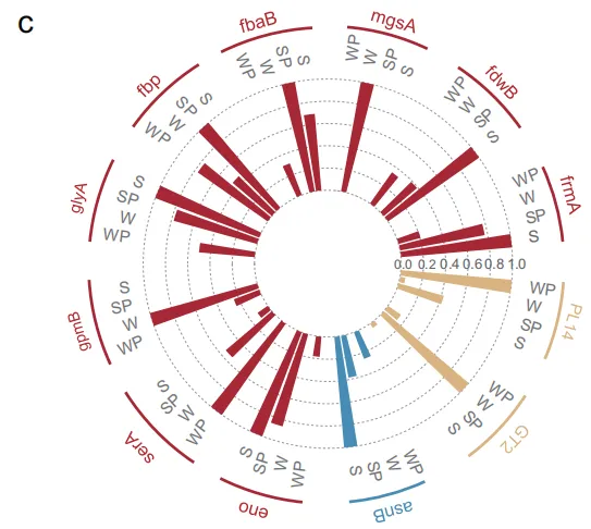
论文原图 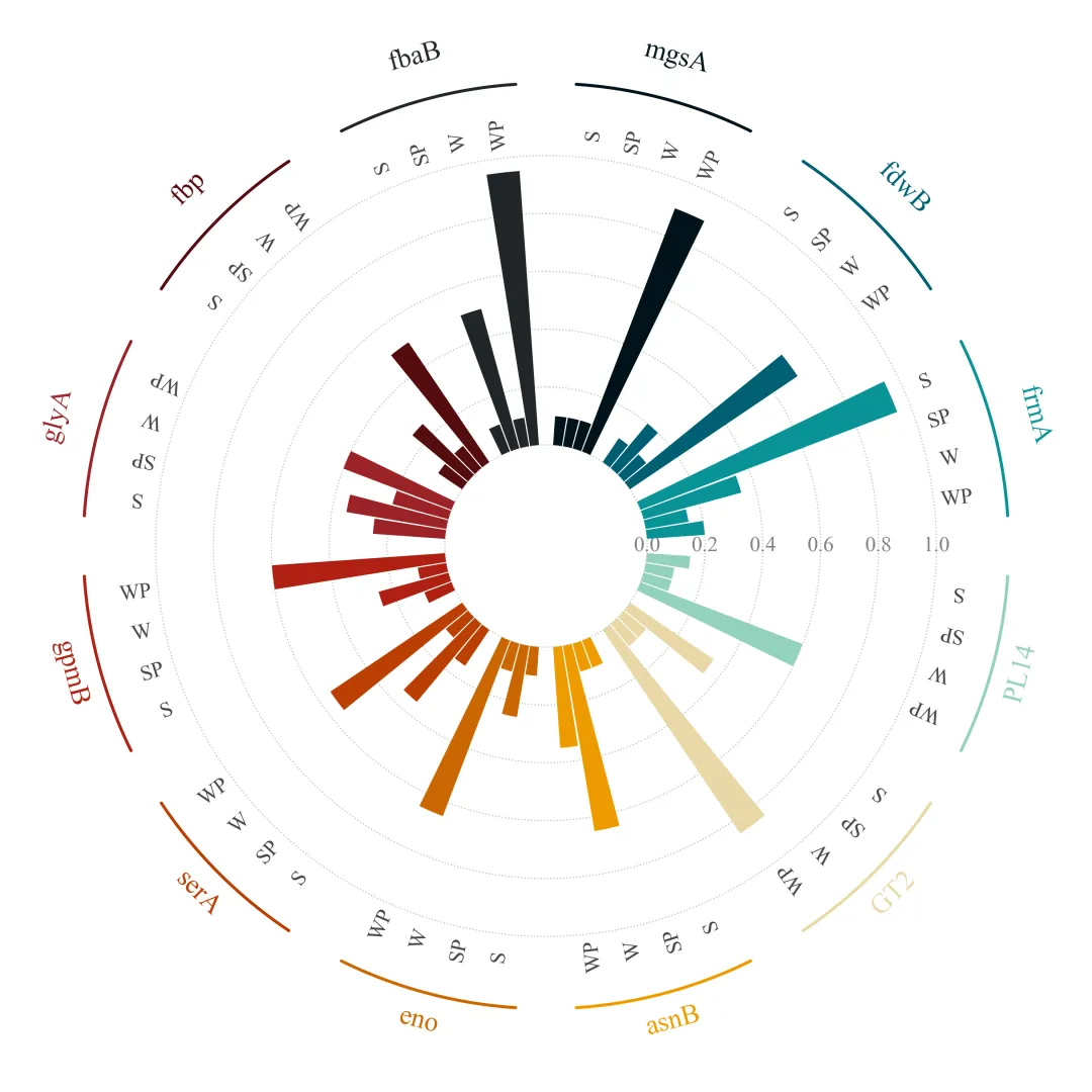
仿图 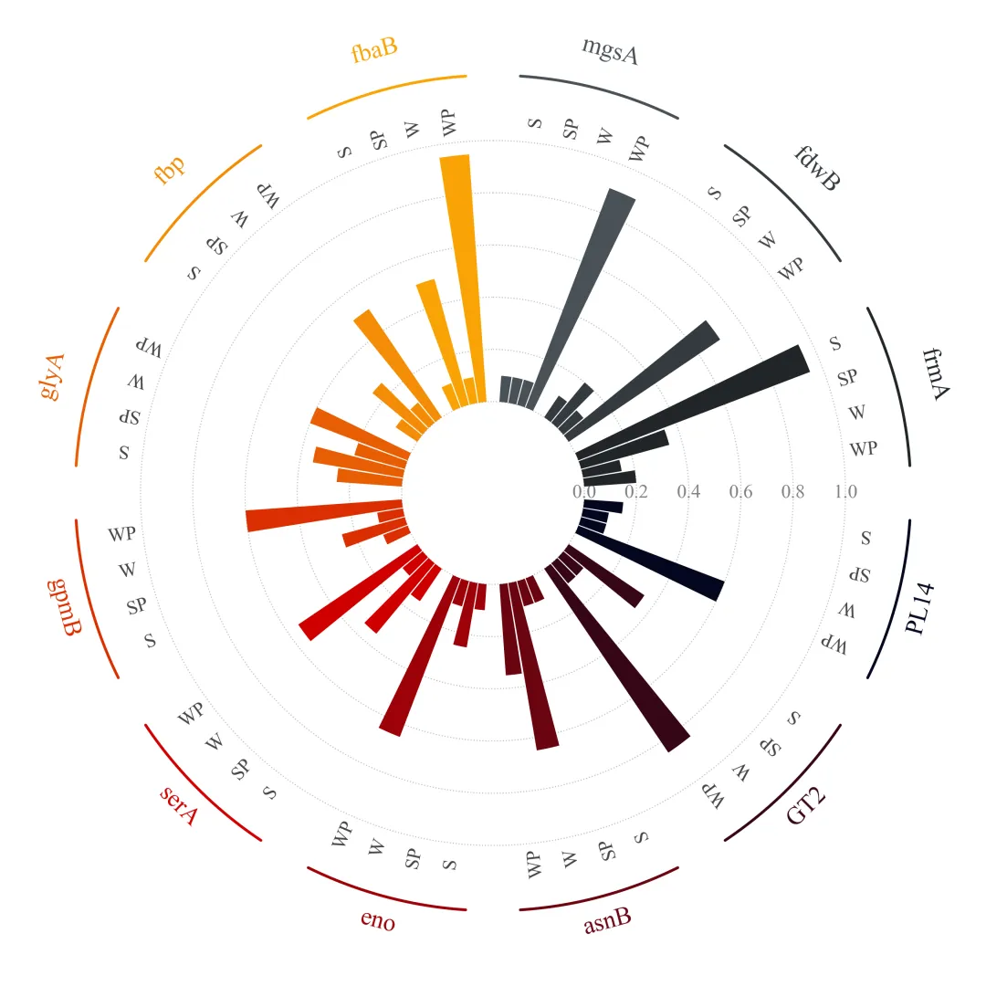
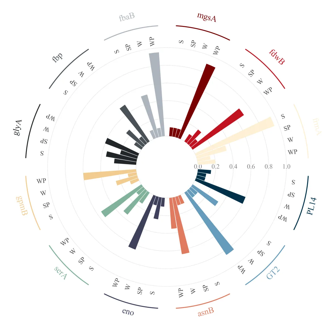
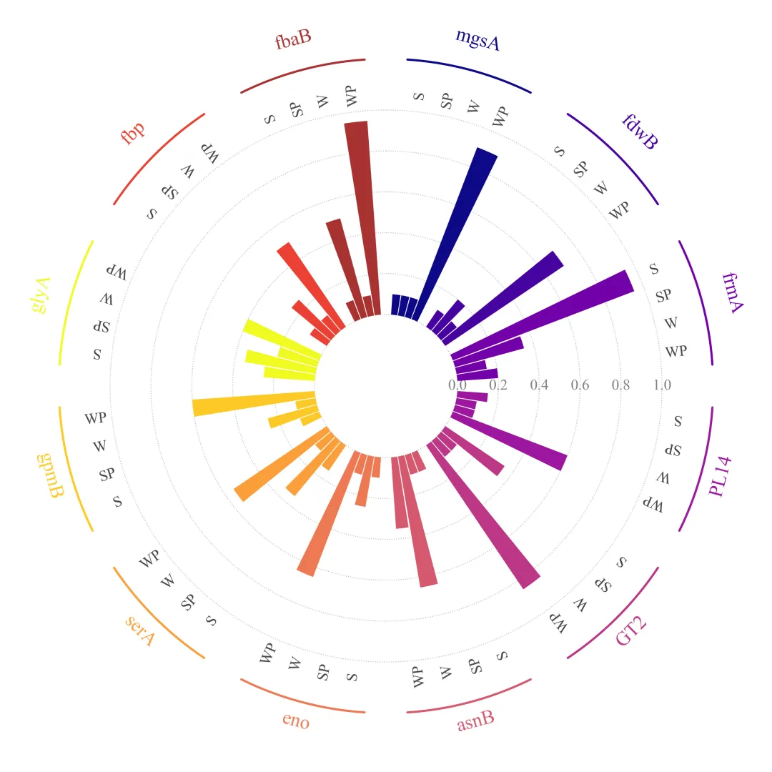
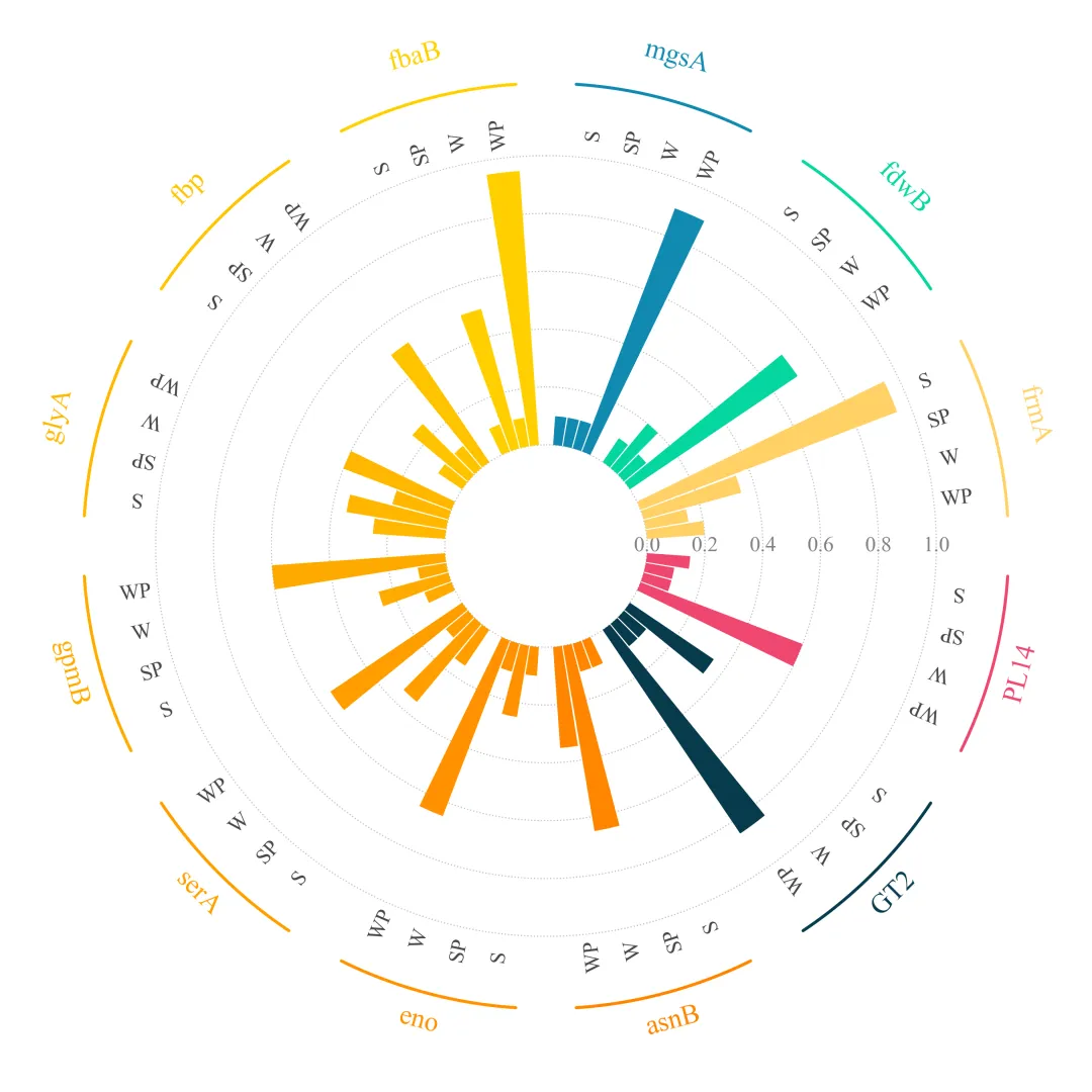
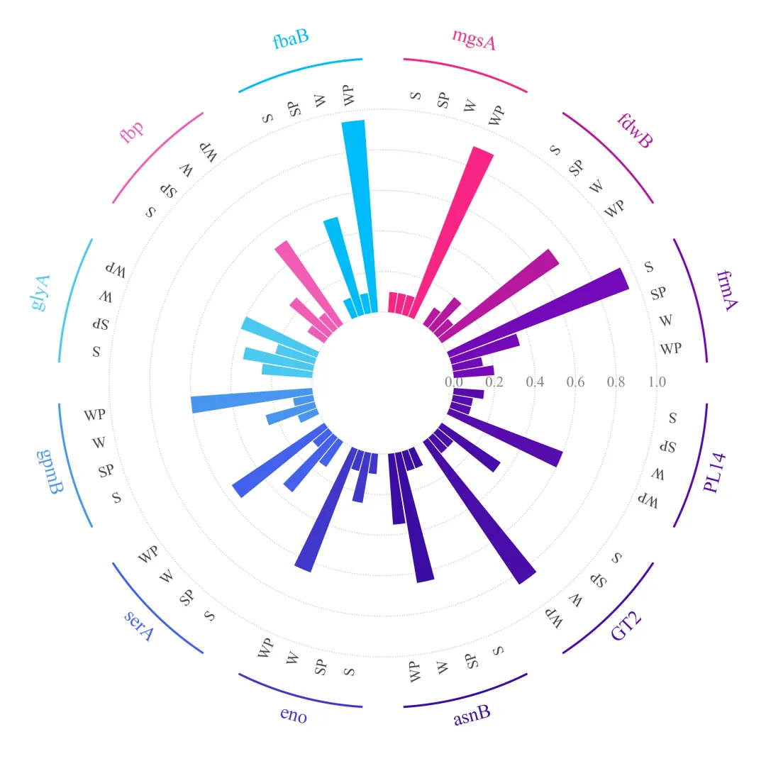
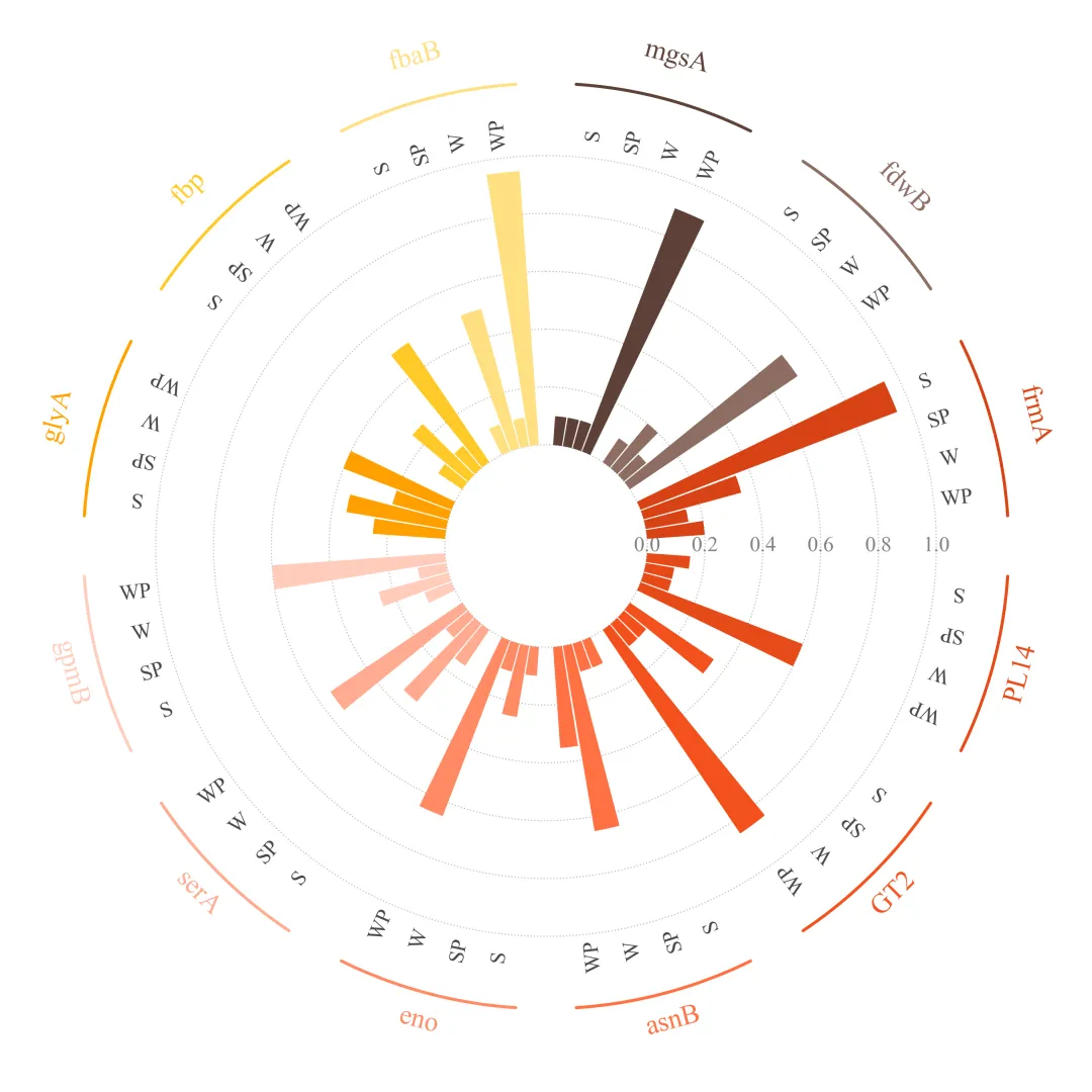
多种配色 


库的导入以及字体设置 
颜色库的设置以及配色方案的选择 
绘图函数:角度计算与数据准备,将一个圆周平均分给每个区域。定义了不同区域之间的空白区域大小。计算出每一根小柱子具体角度,以及每个区域标签的中心位置。 
绘图函数:画布初始化与网格线绘制,设置极坐标,极坐标0度位置,角度增长方向。手动绘制出同心圆虚线。 
绘图函数:绘制柱状图、标签与外圈弧线等。 
执行部分 



期刊图片复现|Python绘制二维偏依赖PDP图 期刊复现|python绘制基于SHAP分析和GAM模型拟合的单特征依赖图 期刊图片复现|python绘制带有渐变颜色shap特征重要性组合图(条形图+蜂巢图) 期刊复现|用Python绘制SHAP特征重要性总览图、依赖图、双特征交互效应SHAP图,解锁XGBoost模型的终极奥秘 期刊图片复现|Python绘制shap重要性蜂巢图+单特征依赖图+交互效应强度气泡图+交互效应依赖图(回归+二分类+分类) 

公众号中的所有所有的免费代码都已经下架了,都并入到付费部分里了,付费合集代码和数据的购买通道已经开通,全部合集100元,后续将会持续更新,决定购买请后台私信我,注意只会分享练习数据和代码文件,不会提供答疑服务,代码文件中已经包含了每行代码的完整注释,购买前请确保真的需要!!!
代码绘制成果展示
代码解释
第一部分
# =========================================================================================# ====================================== 1. 环境设置 =======================================# =========================================================================================import matplotlib.pyplot as pltimport numpy as npimport pandas as pdplt.rcParams['font.family'] = 'serif'plt.rcParams['font.serif'] = ['Times New Roman']plt.rcParams['axes.unicode_minus'] = Falseimport matplotlibmatplotlib.rcParams['pdf.fonttype'] = 42matplotlib.rcParams['ps.fonttype'] = 42
第二部分
# =========================================================================================# ======================================2.颜色库=======================================# =========================================================================================COLOR_LIBRARY = {1: ['#A6CEE3', '#1F78B4', '#B2DF8A', '#33A02C', '#FB9A99', '#E31A1C', '#FDBF6F', '#FF7F00', '#CAB2D6', '#6A3D9A', '#FFFF99', '#B15928'],}SCHEME_ID = 60 #使用的配色方案selected_colors = COLOR_LIBRARY.get(SCHEME_ID, COLOR_LIBRARY[1]) #获取颜色
第三部分
# =========================================================================================# ======================================3.绘图函数=======================================# =========================================================================================def plot_gene_polar_chart(genes, data, conditions, group_colors):num_genes = len(genes) #获取最外圈名称num_conds = len(conditions) #获取柱子数量inner_radius = 0.35 #中间空白半径total_circumference = 2 * np.pi #圆周总弧度sector_angle = total_circumference / num_genes #每个区域的扇形角度gap_ratio = 0.25 #区域之间的间隙比例group_angle_width = sector_angle * (1 - gap_ratio) #实际绘图区域的角度宽度bar_width = group_angle_width / num_conds #柱子的宽度centering_offset = (sector_angle * gap_ratio) / 2 #计算偏移量,使柱子组居中theta = group_start + centering_offset + j * bar_width + bar_width / 2 #当前柱子的中心角度group_thetas.append(theta) #将计算好的角度保存thetas.append(group_thetas) #保存当前区域的所有柱子角度gene_center = group_start + sector_angle / 2 #计算该区域扇形区域的中心角度,用于放置标签gene_centers.append(gene_center) #保存中心角度
第四部分
#创建画布fig = plt.figure(figsize=(10, 10), dpi=150)#添加子图,设置为极坐标投影ax = fig.add_subplot(111, projection='polar')#遍历每一个刻度值for g in grid_values:#绘制背景网格线ax.plot(np.linspace(0, 2 * np.pi, 200), # 生成0到2π的点[inner_radius + g] * 200, #生成对应的半径值color='gray', #颜色linestyle=':', #样式linewidth=0.8, #宽度alpha=0.5, #透明度zorder=0) #顺序
第五部分
#再次遍历每一个区域进行绘图for i in range(num_genes):#获取颜色color = group_colors[i % len(group_colors)]vals = data[i] #获取当前区域对应的数据值angles = thetas[i] #获取当前区域对应的柱子角度label_r = inner_radius + 1.08 #柱子上方标签的半径位置deg = np.degrees(angles[j]) #将弧度转换为角度standard_deg = 90 - deg #转换角度坐标系if 90 < deg < 270:rot = standard_deg + 180 #旋转角度va = 'center' #对齐方式else:rot = standard_deg #旋转角度va = 'center' #对齐方式#添加文本ax.text(angles[j], #角度label_r, #半径conditions[j], #内容rotation=rot, #旋转角度ha='center', #水平居中va=va, #垂直居中fontsize=14, #字体大小color='#444444') #颜色name_r = arc_r + 0.15 #计算区域名称标签的半径位置deg_center = np.degrees(center) % 360 #将中心弧度转换为度角度if 90 < deg_center < 270:name_rot = -deg_center + 180 #旋转角度adj_r = name_r - 0.05 #半径else:name_rot = -deg_center #旋转角度adj_r = name_r #半径#弧线处文本ax.text(center, #中心角度adj_r, #半径genes[i], #文本内容rotation=name_rot, #旋转角度ha='center', #水平居中va='center', #垂直居中fontsize=18, #字体大小color=color) #颜色
第六部分
# =========================================================================================# ======================================4.执行部分=======================================# =========================================================================================if __name__ == "__main__":excel_filename = r"data.xlsx" #数据路径df_read = pd.read_excel(excel_filename) #读取genes_plot = df_read['Gene'].tolist() #最外圈名称conditions = ['S', 'SP', 'W', 'WP'] #柱子数据列data_plot = df_read[conditions].values.tolist() #提取数据并转换为列表#调用绘图函数plot_gene_polar_chart(genes_plot, data_plot, conditions, selected_colors)
如何应用到你自己的数据
1.设置配色:
SCHEME_ID = 60 #使用的配色方案2.设置绘图结果的保存地址:
plt.savefig(fr'result_chart{SCHEME_ID}.png', dpi=300, bbox_inches='tight')3.设置绘图结果的保存地址:
excel_filename = r"\data.xlsx" #数据路径4.提取数据:
genes_plot = df_read['Gene'].tolist() #最外圈名称conditions = ['S', 'SP', 'W', 'WP'] #柱子数据列
推荐
获取方式
本文来自网友投稿或网络内容,如有侵犯您的权益请联系我们删除,联系邮箱:596563534@qq.com 。
随机文章
-
 10个月宝宝每天需要喝多少奶粉?
- Python爬虫入门与合规实操:避开反爬雷区,讲解requests+BeautifulSoup基础用法,实战爬取公开合规数据(如博客文章、公开数据集)
- 重要发布 | 用于开发和控制基于 Python 的立方体卫星平台 —— 智链卫星公司核心软件技术体系
- Python面向对象编程(OOP)通俗解析:告别晦涩概念,用“手机类、学生类”等生活化例子,拆解类、对象、继承、封装的核心逻辑
- 一周练完这70个项目,你的Python就了
- NOAI奥赛官方指定Python春季课程!直击LMCC认证高效夺奖!
- 学python进步蕞快得方式!【自学版】
- Python 线程,进程,多线程,多进程以及并行执行for循环
- 学Python全栈固定80%学习动作,真的能高效
- 学Python这6个自动化办公脚本,告别加班!
- Python仍居第一,但挑战者正在出现!TIOBE 2月榜单发布