Python:从随机实验到双重机器学习
- 2026-06-30 20:28:51
👇 连享会 · 推文导航 | www.lianxh.cn
🍓 课程推荐:连享会 · 2026寒假论文班
嘉宾:郭士祺(上海交通大学)
时间:2026 年 2 月 7-9 日
咨询:王老师 18903405450(微信)

郭老师会带大家拆解 4-5 篇顶刊论文,其中有 3 篇出自他本人之手。
论文班的目标也很明确:不是“听完觉得懂了”,而是让大家学会一套设计因果识别策略的思路和框架,能在研究设计和论文写作中把最核心的问题讲清楚:识别威胁源自哪里、如何进入估计并扭曲解释;你的识别策略依赖哪些关键条件;哪些证据能真正支撑这些条件;哪些不确定性需要在论文里坦诚而规范地呈现。
学完之后,你会更清楚自己论文该怎么搭结构、怎么补证据、怎么回应质疑。

作者:王卓 (合肥工业大学)邮箱:2020171526@mail.hfut.edu.cn
温馨提示: 文中链接在微信中无法生效。请点击底部「阅读原文」。或直接长按/扫描如下二维码,直达原文:

目录
1. 简介
2. 案例背景及相关准备
2.1 案例背景
2.2 DML 估计原理和步骤
2.3 Python 第三方库安装准备
3. 代码操作
3.1 样本、变量说明和数据处理
3.2 原始模型构建
3.3 DML 模型构建
3.4 结果输出
4. 总结
5. 参考资料
6. 相关推文
1. 简介
在经济学中运用因果推断开展研究不可避免会受到混淆变量 (Confounding Variable) 的影响。传统的因果推断方法如双重差分 (DID)、断点回归 (RDD) 等存在一定的局限性,例如解释变量维数过高时的高维陷阱,需要预先设定协变量的函数形式等。
双重机器学习 (Double Machine Learning, DML) 弥补了传统因果估计方法和机器学习方法的缺点。它通过正则化对高维变量选择,正交化解决偏差,样本交叉验证避免过拟合,并对整个估计方法构造置信区间,这在处理经济变量之间的非线性关系等方面具有极大优势。
本文基于微软研究院开发的机器学习因果推断的 Python 第三方库 EconML 和应用案例,展示 DML 方法的使用。
2. 案例背景及相关准备
2.1 案例背景
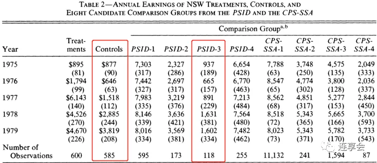
LaLonde (1986) 研究了一项就业培训计划 NSW (The National Supported Work Demonstration),对比该计划对收入的影响在随机实验和非实验数据研究下的差距。NSW 计划旨在通过提供职业培训,帮助美国弱势工人走上长期工作岗位。该培训项目针对的是符合某些条件的男性和女性工人,如正在领取联邦福利金 (AFDC) 或曾经被监禁过。
参加 NSW 项目是自愿的,若一旦选择加入,NSW 就会随机分配他们接受培训 (Treatment group) 或作为对照样本 (Control group),用随机实验评估项目效果。但由于实验成本高,通常情况下,研究人员会使用非实验数据进行项目评估,上述设定也为从非实验数据中捕获因果效应提供了良好环境。
具体步骤为:首先,通过比较 NSW 项目中 Treatment group 和 Control group 来估计项目的效果。虽然工人选择是否参与该计划并不随机,可能与一些个人特征相关,但因为这些工人是随机分配的,所以不用担心任何混杂因素,可以将随机实验的估计值作为真实因果效应的基准。
然后,将 NSW 样本中的 Treatment group 与其他数据集 (非实验数据):the Panel Study of Income Dynamics (PSID) 和 the Current Population Survey (CPS) 中的工人进行比较,重新评估培训的效果。这些非实验数据的工人特征与 NSW 项目的 Control group 存在较大差异,说明从观察数据 (非实验数据) 估计因果关系较为困难。
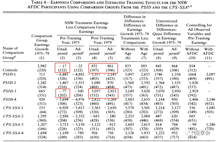
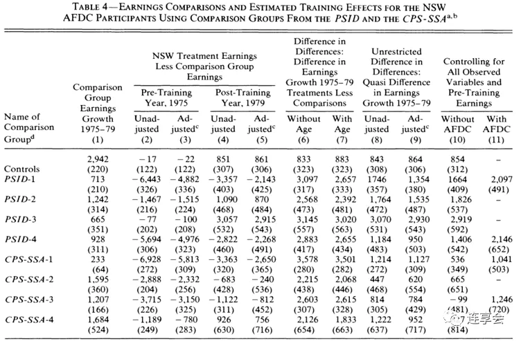
例如,比较 NSW 的 Control group 和 PSID-3 对照组,可以发现这两组人的特征几乎相同 (Table 2 的第 2 列 Controls 和第 5 列的 PSID-3),他们的未经调整和调整的培训前收入也几乎相同 (Table 4 的第 2 列和第 3 列)。在每种情况下,Table 4 第 5 列似乎是处理效应的无偏估计。然而,经过相同的检验,我们发现非实验数据的估计比实验结果多出大约 2100 美元。
2.2 DML 估计原理和步骤
2.2.1 DML 估计原理和模型
是实验影响的被解释变量; 代表样本是否受到实验干预,通常是 0、1 虚拟变量; 是协变量,代表未被实验干预过的个体特征,通常是高维向量。通常情况下,我们直接构建线性回归模型,即用 和 对 回归,估计 的系数,这种方法假定了我们已知晓 的分布。
事实上,高维的 可能内部存在共线性,与 是非线性关系,若单纯的用线性模型进行估计,会存在偏误。此时,我们应用机器学习非线性模型估计 的分布,其中 和 为机器学习模型。
具体地,我们定义 ,即 ,可以推出 。所以估计 需要 和 ,也即估计 和 ,可以利用 Lasso、ANN (人工神经网络)、Random Forest (随机森林) 等机器学习方法拟合这两个期望函数。
2.2.2 DML 估计步骤
运用 DML 进行估计主要有 4 个步骤:
Step 1:将数据集分为 K 个子样本 ,即进行 K 折交叉验证。 Step 2:在 K-1 个子集上训练 的函数形式,在剩余的子集上得到残差 。 Step 3:在 K-1 个子集上训练 的函数形式,在剩余的子集上得到残差 。 Step 4:重复 Step 2-3 K 次,然后遵循 Frisch-Waugh-Lovell 定理,用 对 回归,得到的系数即为 的估计。
2.3 Python 第三方库安装准备
本案例用到了以下第三方库,均采用 pip 安装。主要用 statsmodels 进行论文原始方法的回归,用 econml 和 sckit-learn 实现 DML 。
$pip install econml$pip install pandas$pip install numpy$pip install statsmodels$pip install seaborn$pip install sckit-learn$pip install lightgbm$pip install tqdm$pip install matplotlib3. 代码操作
3.1 样本、变量说明和数据处理
3.1.1 读取数据
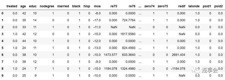
首先读入数据,并大致查看数据的内容。第一个读取的数据集 female_data 为 NSW 女性实验数据,male_data 为 NSW 男性实验数据。其中,female_data 包含了女性 PSID 数据,男性的 PSID 和 CPS 数据进行了额外读取。
# 导入数据处理pandas库import pandas as pd# 若使用Jypter,设置显示所有输出from IPython.core.interactiveshell import InteractiveShellInteractiveShell.ast_node_interactivity = 'all'# 读入数据female_data = pd.read_csv('https://msalicedatapublic.blob.core.windows.net/datasets/Lalonde/calonico_smith_all.csv')male_data = pd.read_csv('https://msalicedatapublic.blob.core.windows.net/datasets/Lalonde/smith_todd.csv')male_cps1 = pd.read_csv('https://msalicedatapublic.blob.core.windows.net/datasets/Lalonde/cps_controls.csv')male_psid1 = pd.read_csv('https://msalicedatapublic.blob.core.windows.net/datasets/Lalonde/psid_controls.csv')male_cps3 = pd.read_csv('https://msalicedatapublic.blob.core.windows.net/datasets/Lalonde/cps_controls3.csv')male_psid3 = pd.read_csv('https://msalicedatapublic.blob.core.windows.net/datasets/Lalonde/psid_controls3.csv')# 展示数据for df in [female_data,male_data,male_psid1,male_psid3,male_cps1,male_cps3]: print(df.head(10))下图展示的为 female_data 数据集前 10 行的部分内容:
其中,核心变量定义如下表所示:
| treated | ||
| age | ||
| educ | ||
| nodegree | ||
| black | ||
| hisp | ||
| married | ||
| haschild | ||
| nchildren75 | ||
| afdc75 | ||
| re74 | ||
| re75 | ||
| re78 | ||
| re79 |
对男性和女性数据的官方描述性统计如下方表格所示:
描述性统计 (男性)
| age | ||||||
| educ | ||||||
| nodegree | ||||||
| black | ||||||
| hisp | ||||||
| married | ||||||
| re74 | ||||||
| re75 | ||||||
| re78 | ||||||
| N |
描述性统计 (女性)
| age | ||||
| educ | ||||
| nodegree | ||||
| black | ||||
| hisp | ||||
| married | ||||
| haschild | ||||
| nchildren75 | ||||
| afdc75 | ||||
| re74 | ||||
| re75 | ||||
| re79 | ||||
| N |
3.1.2 处理数据
对读入的数据进行初步处理,主要是进行分割数据集的操作。
## femalefemale_data["haschild"]=(female_data["nchildren75"]>0)*1female_data = female_data[pd.notnull(female_data.re75) & pd.notnull(female_data.re79)]female_treatment = female_data[female_data.treated==1.].copy()female_control = female_data[female_data.treated==0.].copy()female_psid1 = female_data[female_data['psid1']==1].copy()female_psid2 = female_data[female_data['psid2']==1].copy()### 处理数据female_psid1.loc[:, 'treated'] = 0female_psid2.loc[:, 'treated'] = 0## malemale_treatment = male_data[male_data.treated==1.].copy()male_control = male_data[male_data.treated==0.].copy()### 处理数据 (统一名称) for df in [male_psid1,male_psid3,male_cps1,male_cps3]: df.rename(columns={'treat':'treated', 'education':'educ', 'hispanic':'hisp'}, inplace=True)3.1.3 整合数据
对所有变量进行整合,方便后续模型处理和图像展示。
# outcomeoutcome_name_male="re78"outcome_name_female="re79"# ols controlsbasic_ols_columns = ['treated', 'age', 'age_2', 'educ', 'nodegree', 'black', 'hisp']complete_ols_columns_male = basic_ols_columns+["married","re75","re75_dummy", \"re74","re74_dummy","re_diff_pre"]complete_ols_columns_female=basic_ols_columns+["married","re75","re75_dummy", \"re74","re74_dummy", "re_diff_pre","afdc75","nchildren75","haschild"]# econml controls (exclude treatment)econml_controls_male= ['age', 'age_2', 'educ', 're75','re74','re_diff_pre','nodegree', \'black', 'hisp', 'married', 're75_dummy','re74_dummy']econml_controls_female= ['age', 'age_2', 'educ','nchildren75', 're75','re74','re_diff_pre', \'nodegree', 'black', 'hisp', 'married','re75_dummy','re74_dummy','afdc75','haschild']defpreprocessing(df,outcome_name,column_names):# add indicator of zero earnings df["re74_dummy"]=(df["re74"]>0)*1 df["re75_dummy"]=(df["re75"]>0)*1# get growth of pre training earning df["re_diff_pre"]=df["re75"]-df["re74"]# add age square df["age_2"]=df["age"]**2# select columns df=df[column_names+[outcome_name]]return df# preprocessing datamale_control, male_treatment, male_psid1, male_psid3, male_cps1, male_cps3 \ = [preprocessing(df,outcome_name_male,complete_ols_columns_male) \for df in (male_control, male_treatment, male_psid1, \ male_psid3, male_cps1, male_cps3)]female_control, female_treatment, female_psid1, female_psid2 \ =[preprocessing(df,outcome_name_female,complete_ols_columns_female)\for df in (female_control, female_treatment, female_psid1, female_psid2)]3.2 原始模型构建
接下来,我们用 statsmodels 库构建 OLS 模型,对论文原始结果进行复现。
import statsmodels.api as smdefols_reg_wrapper(reg_data, x_columns, y_column, print_summary=False):""" 输入: reg_data:整个数据集 x_column:解释变量列 y_column:被解释变量 输出: effect:treated系数 se:标准误 lb、ub:置信区间上下界 """ X = reg_data[x_columns].values X = pd.DataFrame(sm.add_constant(X,has_constant='add'),columns=["intercept"]+x_columns) Y = reg_data[y_column] model = sm.OLS(Y, X, hasconst=True) results = model.fit()# save results for summary table effect = int(round(results.params['treated'])) se = int(round(results.bse['treated'])) lb=int(round(results.conf_int().loc["treated"][0])) ub=int(round(results.conf_int().loc["treated"][1]))if print_summary: print(results.summary())return effect, se, lb, ub3.3 DML 模型构建
这部分,我们首先定义两个函数,first_stage_reg 和 first_stage_clf,分别表示了 DML 估计步骤的 Step 2 和 Step 3。每个步骤的机器学习模型,在 Lasso (拉索)、Random Forest (随机森林)、LigthGBM (一种梯度提升决策树) 等模型中,通过 GridSearchCVList 选择最优模型和参数。
from sklearn.linear_model import LogisticRegressionCV, \ LinearRegression,LogisticRegression,Lasso,LassoCVfrom sklearn.ensemble import RandomForestClassifier, \ RandomForestRegressor,GradientBoostingClassifierimport lightgbm as lgbfrom sklearn.preprocessing import StandardScalerfrom econml.sklearn_extensions.model_selection import GridSearchCVListdeffirst_stage_reg(X, y, *, automl=True):if automl: model = GridSearchCVList([LassoCV(), RandomForestRegressor(n_estimators=100), lgb.LGBMRegressor()], param_grid_list=[{}, {'max_depth': [5,10,20],'min_samples_leaf': [5, 10]}, {'learning_rate': [0.02,0.05,0.08], 'max_depth': [3, 5]}], cv=3, scoring='neg_mean_squared_error') best_est = model.fit(X, y).best_estimator_if isinstance(best_est, LassoCV):return Lasso(alpha=best_est.alpha_)return best_estelse: model = LassoCV(cv=5).fit(X, y)return Lasso(alpha=model.alpha_)deffirst_stage_clf(X, y, *, make_regressor=False, automl=True):if automl: model = GridSearchCVList([LogisticRegressionCV(max_iter=1000), RandomForestClassifier(n_estimators=100), lgb.LGBMClassifier()], param_grid_list=[{}, {'max_depth': [5,10,20],'min_samples_leaf': [5, 10]}, {'learning_rate':[0.01,0.05,0.1],'max_depth': [3,5]}], cv=3, scoring='neg_log_loss') est = model.fit(X, y).best_estimator_if isinstance(est,LogisticRegressionCV):return LogisticRegression(C=est.C_[0])else: model = LogisticRegressionCV(cv=5, max_iter=1000).fit(X, y) est = LogisticRegression(C=model.C_[0])if make_regressor:return _RegressionWrapper(est)else:return est在选择出最优模型和参数后,我们使用 econml 进行 DML 模型构建。
import numpy as npfrom econml.dml import LinearDMLfrom econml.dr import LinearDRLearnerdefeconml_homo_model_wrapper(reg_data, control_names,outcome_name, \ model_type,*,cols_to_scale, print_summary=False):# get variables X = None# no heterogeneous treatment W = reg_data[control_names].values# scale W scaler = StandardScaler() W = np.hstack([scaler.fit_transform(W[:, :cols_to_scale]).astype(np.float32), W[:, cols_to_scale:]]) T = reg_data["treated"] y = reg_data[outcome_name]# select the best nuisances model out of econml estimator model_y=first_stage_reg(W, y) model_t=first_stage_clf(W, T)if model_type=='dml': est = LinearDML(model_y=model_y, model_t=model_t, discrete_treatment=True, mc_iters=5,cv=5)elif model_type=='dr': est = LinearDRLearner(model_regression=model_y, model_propensity=model_t, mc_iters=5,cv=5)else:raise ValueError('invalid model type %s' % model_type)try: est.fit(y, T, X=X, W=W, inference="statsmodels")except np.linalg.LinAlgError as e: est.fit(y, T, X=X, W=W, inference="statsmodels")# Get the final coefficient and intercept summaryif model_type=="dml": inf=est.intercept__inference()else: inf=est.intercept__inference(T=1) effect=int(round(inf.point_estimate)) se=int(round(inf.stderr)) lb,ub=inf.conf_int(alpha=0.05)if print_summary:if model_type=='dml': print(est.summary(alpha=0.05))else: print(est.summary(T=1,alpha=0.05))return effect, se, int(round(lb)), int(round(ub))最后,定义函数 get_summ_table 将所有回归的结果进行输出
from tqdm import tqdmdefget_summ_table(dfs,treat_df,*,df_names,basic_ols_controls, \ complete_ols_controls,econml_controls,outcome_name,cols_to_scale): summ_dic={"control_name":[],"# of obs":[],"earning_growth":[],"OLS":[], \"OLS full controls":[],"DML full controls":[]} summ_dic1={"control_name":[],"method":[],"point_estimate":[],"stderr":[],\"lower_bound":[],"upper_bound":[]}for df, name in tqdm(zip(dfs, df_names)): summ_dic["control_name"].append(name) summ_dic["# of obs"].append(df.shape[0]) summ_dic1["control_name"]+=[name]*3# get table 5 col 1 growth=int(np.round((df[outcome_name]-df["re75"]).mean(),0)) summ_dic["earning_growth"].append(growth)# get table 5 col 5 summ_dic1["method"].append("OLS") df_all=pd.concat([treat_df,df],axis=0,ignore_index=True) effect,se,lb,ub=ols_reg_wrapper(df_all,basic_ols_controls,outcome_name,print_summary=False) summ_dic["OLS"].append([effect,se]) summ_dic1["point_estimate"].append(effect) summ_dic1["stderr"].append(se) summ_dic1["lower_bound"].append(lb) summ_dic1["upper_bound"].append(ub)# get table 5 col 10 summ_dic1["method"].append("OLS full controls") effect,se,lb,ub=ols_reg_wrapper(df_all,complete_ols_controls,outcome_name,print_summary=False) summ_dic["OLS full controls"].append([effect,se]) summ_dic1["point_estimate"].append(effect) summ_dic1["stderr"].append(se) summ_dic1["lower_bound"].append(lb) summ_dic1["upper_bound"].append(ub)# dml summ_dic1["method"].append("DML full controls") effect,se,lb,ub=econml_homo_model_wrapper(df_all, econml_controls, \ outcome_name,"dml",cols_to_scale=cols_to_scale, print_summary=False) summ_dic["DML full controls"].append([effect,se]) summ_dic1["point_estimate"].append(effect) summ_dic1["stderr"].append(se) summ_dic1["lower_bound"].append(lb) summ_dic1["upper_bound"].append(ub) return summ_dic,summ_dic13.4 结果输出
这里,我们将上述模型结果输出,并对比 Lalonde (1986) 文中 ATE 的估计。
3.4.1 男性处理效应的对比
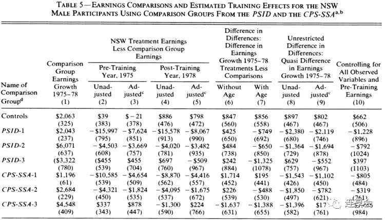
control_dfs_male=[male_control,male_psid1,male_psid3,male_cps1,male_cps3]df_names_male=["exp controls","psid1","psid3","cps1","cps3"]summ_male,summplot_male=get_summ_table(control_dfs_male,male_treatment,df_names=df_names_male, basic_ols_controls=basic_ols_columns, complete_ols_controls=complete_ols_columns_male, econml_controls=econml_controls_male, outcome_name=outcome_name_male,cols_to_scale=6 )summ_male_df=pd.DataFrame(summ_male)summ_male_df其中,中括号中的数值分别代表点估计和标准误。原文中的估计结果如下图所示:
然后,绘制每种估计方法的误差条图。
import matplotlib.pyplot as pltfrom matplotlib.transforms import ScaledTranslation%matplotlib inlinedefplot_errorbar(df,df_names): fig, ax = plt.subplots(figsize=(10,6))for ind,control_name in enumerate(df_names): sub_df=df[df["control_name"]==control_name] method_name=sub_df["method"].values point=sub_df["point_estimate"].values yerr=np.zeros((2,point.shape[0])) yerr[0,:]=point-sub_df["lower_bound"].values yerr[1,:]=sub_df["upper_bound"].values-point trans = ax.transData + ScaledTranslation((-10+ind*5)/72, 0, fig.dpi_scale_trans) plt.errorbar(method_name,point,yerr,fmt="o",capsize=5, \ elinewidth=2,label=control_name,alpha=0.7,transform=trans) plt.axhline(y=0, color='black', linestyle='--',alpha=0.5) plt.legend() plt.xlabel("Methodology") plt.ylabel("ATE with CI") plt.title("Error bar of each method for each dataset") plt.show()summplot_male_df=pd.DataFrame(summplot_male)plot_errorbar(summplot_male_df,df_names_male)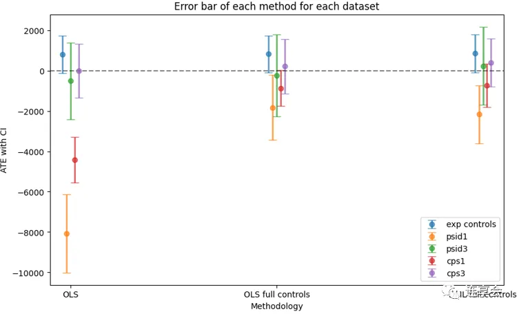
3.4.2 女性处理效应的对比
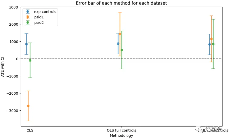
同理,女性处理效应对比和误差条代码如下所示:
control_dfs_female=[female_control,female_psid1,female_psid2]df_names_female=["exp controls","psid1","psid2"]summ_female,summplot_female=get_summ_table(control_dfs_female,female_treatment,df_names=df_names_female, basic_ols_controls=basic_ols_columns, complete_ols_controls=complete_ols_columns_female, econml_controls=econml_controls_female, outcome_name=outcome_name_female,cols_to_scale=7 )summ_female_df=pd.DataFrame(summ_female)summ_female_df原文中的估计结果:
4. 总结
根据上述结果可以发现,在一些样本上,如 PSID1、CPS1,双重机器学习 DML 比论文中的传统非实验估计具有更好的表现。以上仅为 EconML 实现 DML 的部分操作,更多细节和用法,可以登录 官网 查看。
5. 参考资料
LaLonde R J. Evaluating the econometric evaluations of training programs with experimental data[J]. The American economic review, 1986: 604-620. -PDF- Econml官方指南 Econml Case Study 双重机器学习:原理、实现步骤与R程序
6. 相关推文
Note:产生如下推文列表的 Stata 命令为:
lianxh 机器学习, m安装最新版lianxh命令:ssc install lianxh, replace
专题:论文写作 Semantic scholar:一款基于机器学习的学术搜索引擎 专题:Stata教程 Stata-Python交互-7:在Stata中实现机器学习-支持向量机 专题:Stata命令 Stata:双重机器学习-多维聚类标准误的估计方法-crhdreg 专题:Python-R-Matlab MLRtime:如何在 Stata 调用 R 的机器学习包? 专题:其它 知乎热议:机器学习在经济学的应用前景 专题:机器学习 知乎热议:如何学习机器学习 机器学习在经济学领域的应用前景 机器学习如何用?金融+能源经济学文献综述 知乎热议:纠结-计量经济、时间序列和机器学习 机器学习:随机森林算法的Stata实现 Stata:机器学习分类器大全

连享会微信小店上线啦!
Note:扫一扫进入“连享会微信小店”,你想学的课程在这里······