🏠 Python数据分析:用线性回归预测房价数据项目实战
大家好!今天带大家完成一个经典的回归分析项目——用线性回归预测房价。我们将通过 Python 的 Pandas、Matplotlib、Seaborn 和 StatsModels 库,对一个真实的房屋交易数据集进行探索、清洗、建模,最后预测一套新房屋的售价。整个过程按步骤展开,代码清晰,结果直观,非常适合新手入门数据分析与机器学习!
🎯 分析目标
我们的目标是:基于已有的房屋销售价格及其属性,建立一个线性回归模型,然后预测以下这套房屋的售价:
❝面积为 6500 平方英尺,4 个卧室、2 个厕所,总共 2 层,不位于主路,无客人房,带地下室,有热水器,没有空调,车位数为 2,位于城市首选社区,简装修。
📁 简介
数据集 house_price.csv 记录了超过 500 栋房屋的交易价格及相关属性,包含以下字段:
| | |
|---|
| | |
| | |
| | |
| | |
| | |
| | |
| | |
| | |
| | |
| | |
| | |
| | |
| | furnished(精装)semi-furnished(简装)unfurnished(毛坯) |
📥 读取数据
首先导入必要的库,并用 Pandas 读取 CSV 文件。
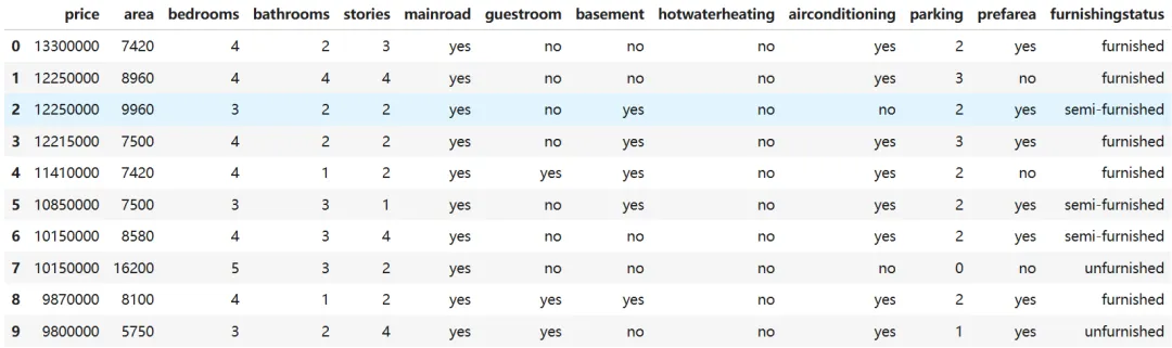
import pandas as pdimport matplotlib.pyplot as pltimport seaborn as snsoriginal_house_price = pd.read_csv("house_price.csv")original_house_price.head()
输出前 5 行:
🧹 评估和清理数据
创建数据副本,保留原始数据。
cleaned_house_price = original_house_price.copy()
📐 数据整齐度
数据已符合“每列一个变量,每行一个观察值”,无需调整。
cleaned_house_price.head(10)
🧽 数据干净度
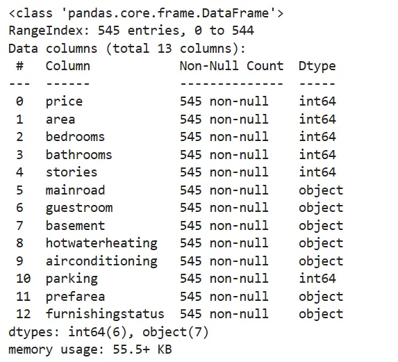
检查数据类型,将分类变量转换为 category 类型。
cleaned_house_price.info()
所有字段均无缺失值(545 条非空)。
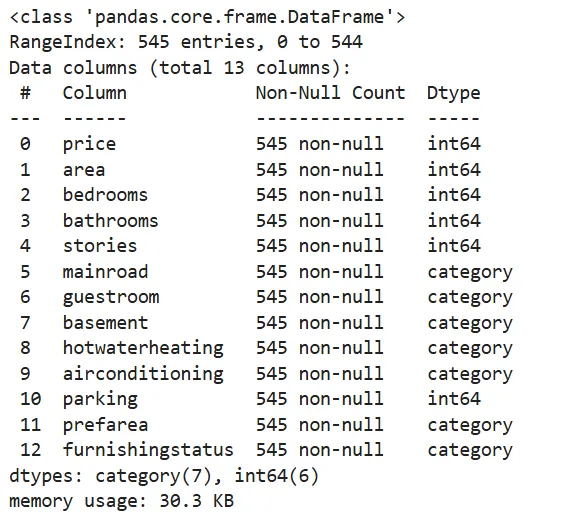
# 类型转换cleaned_house_price['mainroad'] = cleaned_house_price['mainroad'].astype("category")cleaned_house_price['guestroom'] = cleaned_house_price['guestroom'].astype("category")cleaned_house_price['basement'] = cleaned_house_price['basement'].astype("category")cleaned_house_price['hotwaterheating'] = cleaned_house_price['hotwaterheating'].astype("category")cleaned_house_price['airconditioning'] = cleaned_house_price['airconditioning'].astype("category")cleaned_house_price['prefarea'] = cleaned_house_price['prefarea'].astype("category")cleaned_house_price['furnishingstatus'] = cleaned_house_price['furnishingstatus'].astype("category")cleaned_house_price.info()
🔍 处理缺失数据
无缺失值。
🔁 处理重复数据
允许重复,不处理。
⚠️ 处理不一致数据
检查各分类变量的唯一值,均无异常。
cleaned_house_price["mainroad"].value_counts()# yes 468, no 77cleaned_house_price["guestroom"].value_counts()# no 448, yes 97cleaned_house_price["basement"].value_counts()# no 354, yes 191cleaned_house_price["hotwaterheating"].value_counts()# no 520, yes 25cleaned_house_price["airconditioning"].value_counts()# no 373, yes 172cleaned_house_price["prefarea"].value_counts()# no 417, yes 128cleaned_house_price["furnishingstatus"].value_counts()# semi-furnished 227, unfurnished 178, furnished 140
❌ 处理无效或错误数据
用 describe() 查看数值型字段的统计信息,均在合理范围内。
cleaned_house_price.describe()
📊 探索数据
开始可视化探索,先设置配色风格。
sns.set_palette("pastel")
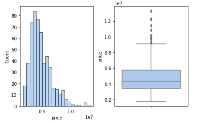
🏷 房价分布
plt.rcParams["figure.figsize"] = [7.00, 3.50]plt.rcParams["figure.autolayout"] = Truefigure, axes = plt.subplots(1, 2)sns.histplot(cleaned_house_price, x='price', ax=axes[0])sns.boxplot(cleaned_house_price, y='price', ax=axes[1])plt.show()
📌 结论:房价呈右偏分布,大多数房屋价格中等,但存在一些高价的极端值。
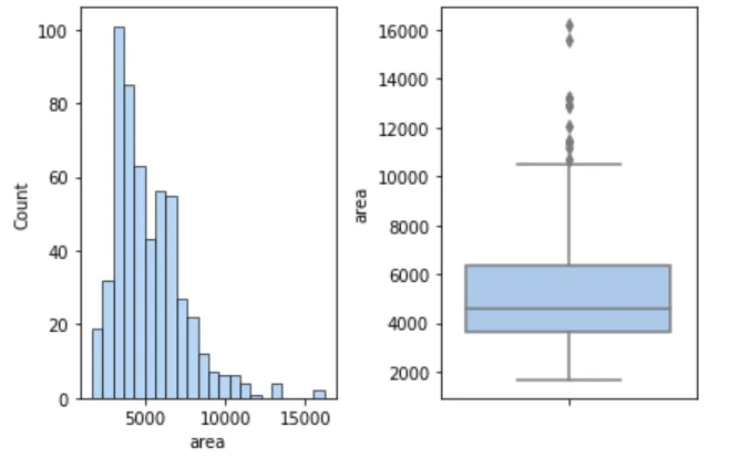
📐 面积分布
figure, axes = plt.subplots(1, 2)sns.histplot(cleaned_house_price, x='area', ax=axes[0])sns.boxplot(cleaned_house_price, y='area', ax=axes[1])plt.show()
📌 结论:面积分布同样右偏,与房价相似。
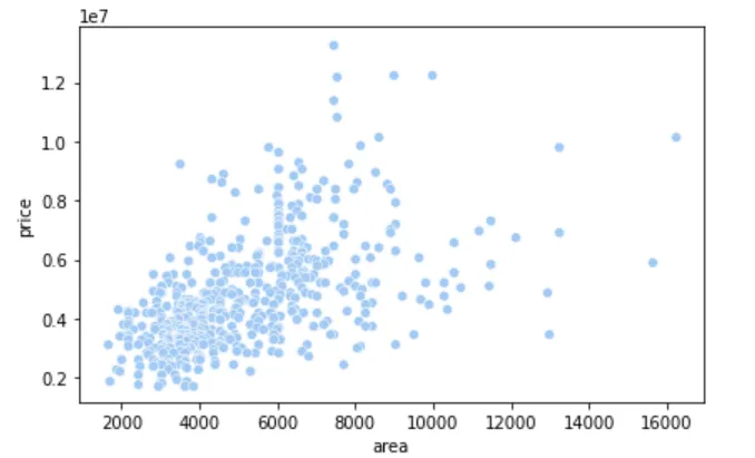
📈 房价与面积的关系
sns.scatterplot(cleaned_house_price, x='area', y='price')plt.show()
📌 结论:散点图显示面积与房价大致呈正相关,但相关性强度需进一步计算。
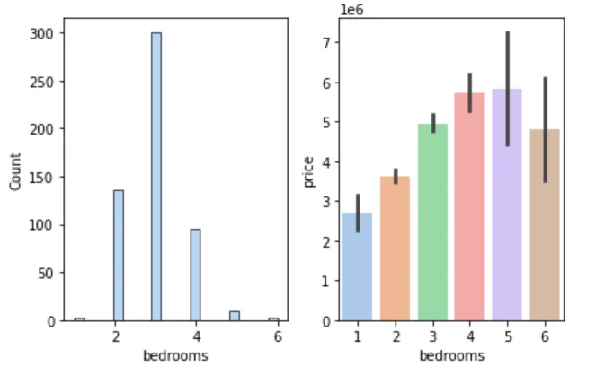
🛏 卧室数与房价
figure, axes = plt.subplots(1, 2)sns.histplot(cleaned_house_price, x='bedrooms', ax=axes[0])sns.barplot(cleaned_house_price, x='bedrooms', y='price', ax=axes[1])plt.show()
📌 结论:卧室数多为 2~4 个,平均房价随卧室数增加而上升,但超过 5 个后不再明显。
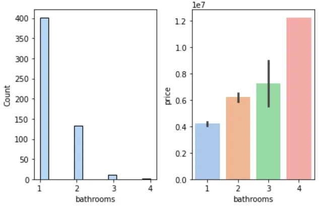
🚽 洗手间数与房价
figure, axes = plt.subplots(1, 2)sns.histplot(cleaned_house_price, x='bathrooms', ax=axes[0])sns.barplot(cleaned_house_price, x='bathrooms', y='price', ax=axes[1])plt.show()
📌 结论:洗手间越多,房价越高。
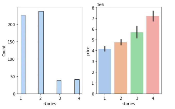
🏢 楼层数与房价
figure, axes = plt.subplots(1, 2)sns.histplot(cleaned_house_price, x='stories', ax=axes[0])sns.barplot(cleaned_house_price, x='stories', y='price', ax=axes[1])plt.show()
📌 结论:楼层越多,房价越高。
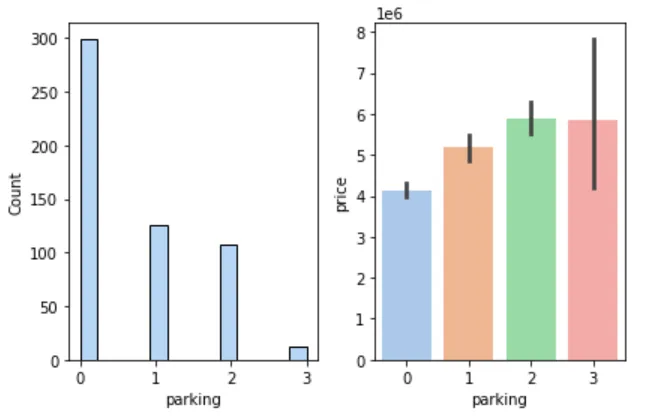
🚗 车库数与房价
figure, axes = plt.subplots(1, 2)sns.histplot(cleaned_house_price, x='parking', ax=axes[0])sns.barplot(cleaned_house_price, x='parking', y='price', ax=axes[1])plt.show()
📌 结论:车库数量增加,房价上升,但超过 2 个后增长放缓。
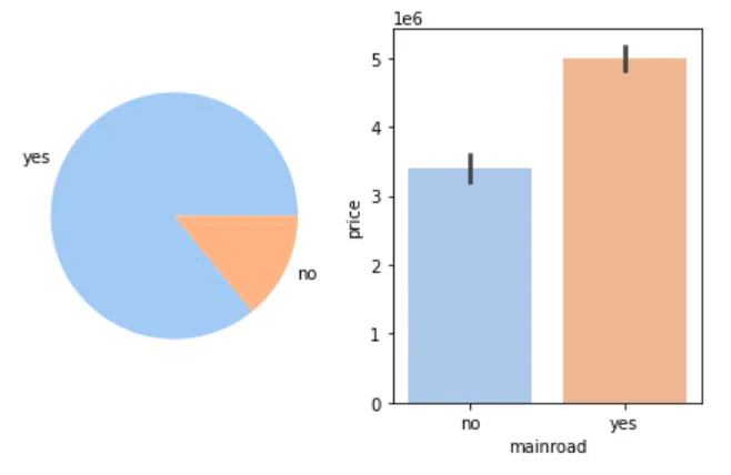
🛣 是否在主路与房价
figure, axes = plt.subplots(1, 2)mainroad_count = cleaned_house_price['mainroad'].value_counts()mainroad_label = mainroad_count.indexaxes[0].pie(mainroad_count, labels=mainroad_label)sns.barplot(cleaned_house_price, x='mainroad', y='price', ax=axes[1])plt.show()
📌 结论:大多数房子位于主路,且平均房价更高。
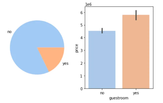
🛋 是否有客人房与房价
figure, axes = plt.subplots(1, 2)guestroom_count = cleaned_house_price['guestroom'].value_counts()guestroom_label = guestroom_count.indexaxes[0].pie(guestroom_count, labels=guestroom_label)sns.barplot(cleaned_house_price, x='guestroom', y='price', ax=axes[1])plt.show()
📌 结论:有客人房的房子价格更高。
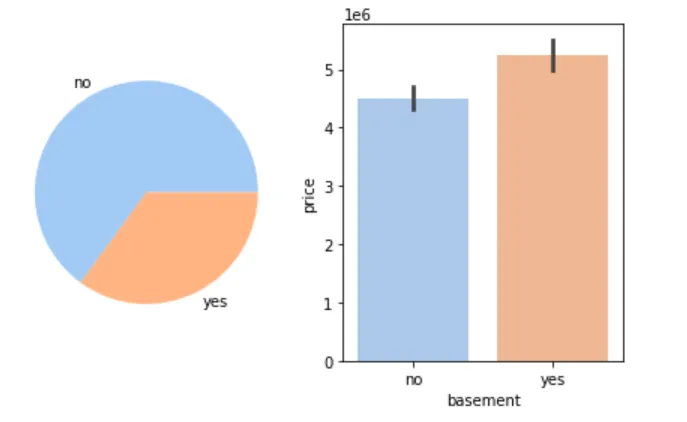
🧱 是否有地下室与房价
figure, axes = plt.subplots(1, 2)basement_count = cleaned_house_price['basement'].value_counts()basement_label = basement_count.indexaxes[0].pie(basement_count, labels=basement_label)sns.barplot(cleaned_house_price, x='basement', y='price', ax=axes[1])plt.show()
📌 结论:有地下室的房子价格更高。
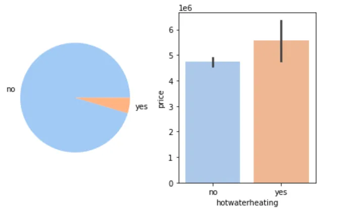
🔥 是否有热水器与房价
figure, axes = plt.subplots(1, 2)hotwaterheating_count = cleaned_house_price['hotwaterheating'].value_counts()hotwaterheating_label = hotwaterheating_count.indexaxes[0].pie(hotwaterheating_count, labels=hotwaterheating_label)sns.barplot(cleaned_house_price, x='hotwaterheating', y='price', ax=axes[1])plt.show()
📌 结论:有热水器的房子价格更高(虽然样本很少)。
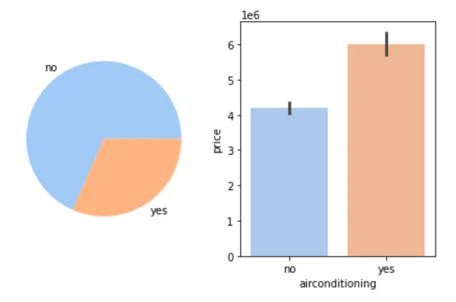
❄️ 是否有空调与房价
figure, axes = plt.subplots(1, 2)airconditioning_count = cleaned_house_price['airconditioning'].value_counts()airconditioning_label = hotwaterheating_count.indexaxes[0].pie(airconditioning_count, labels=airconditioning_label)sns.barplot(cleaned_house_price, x='airconditioning', y='price', ax=axes[1])plt.show()
📌 结论:有空调的房子价格更高。
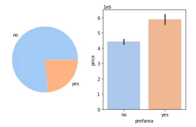
🌆 是否位于城市首选社区与房价
figure, axes = plt.subplots(1, 2)prefarea_count = cleaned_house_price['prefarea'].value_counts()prefarea_label = prefarea_count.indexaxes[0].pie(prefarea_count, labels=prefarea_label)sns.barplot(cleaned_house_price, x='prefarea', y='price', ax=axes[1])plt.show()
📌 结论:位于首选社区的房价更高。
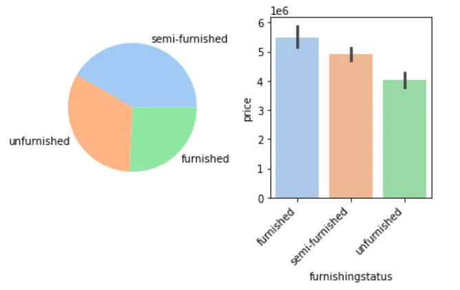
🛋 装修状态与房价
figure, axes = plt.subplots(1, 2)furnishingstatus_count = cleaned_house_price['furnishingstatus'].value_counts()furnishingstatus_label = furnishingstatus_count.indexaxes[0].pie(furnishingstatus_count, labels=furnishingstatus_label)sns.barplot(cleaned_house_price, x='furnishingstatus', y='price', ax=axes[1])axes[1].set_xticklabels(axes[1].get_xticklabels(), rotation=45, horizontalalignment='right')plt.show()
📌 结论:精装 > 简装 > 毛坯,装修越好房价越高。
🔬 分析数据
现在开始构建线性回归模型。使用 statsmodels 库。
import statsmodels.api as sm
创建建模专用副本。
lr_house_price = cleaned_house_price.copy()
🔁 引入虚拟变量
将所有分类变量转换为虚拟变量(独热编码),并丢弃第一类以避免多重共线性。
lr_house_price = pd.get_dummies(lr_house_price, drop_first=True, columns=['mainroad', 'guestroom', 'basement','hotwaterheating', 'airconditioning','prefarea', 'furnishingstatus'], dtype=int)lr_house_price.head()
| | | | | | | | | | | | | furnishingstatus_semi-furnished | furnishingstatus_unfurnished |
|---|
| | | | | | | | | | | | | | |
|---|
| | | | | | | | | | | | | | |
|---|
| | | | | | | | | | | | | | |
|---|
| | | | | | | | | | | | | | |
|---|
| | | | | | | | | | | | | | |
|---|
| | | | | | | | | | | | | | |
|---|
| | | | | | | | | | | | | | |
|---|
| | | | | | | | | | | | | | |
|---|
| | | | | | | | | | | | | | |
|---|
| | | | | | | | | | | | | | |
|---|
| | | | | | | | | | | | | | |
|---|
545 rows × 14 columns
🎯 划分因变量和自变量
y = lr_house_price['price']X = lr_house_price.drop('price', axis=1)
🔍 检查多重共线性
计算自变量之间的相关系数,看是否有绝对值 >0.8 的高度相关变量。
X.corr().abs() > 0.8
| | | | | | | | | | | | furnishingstatus_semi-furnished | furnishingstatus_unfurnished |
|---|
| | | | | | | | | | | | | |
|---|
| | | | | | | | | | | | | |
|---|
| | | | | | | | | | | | | |
|---|
| | | | | | | | | | | | | |
|---|
| | | | | | | | | | | | | |
|---|
| | | | | | | | | | | | | |
|---|
| | | | | | | | | | | | | |
|---|
| | | | | | | | | | | | | |
|---|
| | | | | | | | | | | | | |
|---|
| | | | | | | | | | | | | |
|---|
| | | | | | | | | | | | | |
|---|
| furnishingstatus_semi-furnished | | | | | | | | | | | | | |
|---|
| furnishingstatus_unfurnished | | | | | | | | | | | | | |
|---|
输出显示无强相关性,可以放心使用所有变量。
➕ 添加截距项
X = sm.add_constant(X)
🧮 拟合模型
model = sm.OLS(y, X).fit()model.summary()
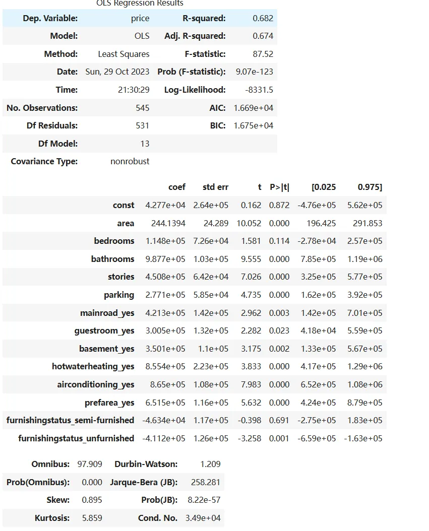 输出结果摘要(部分):
- R-squared = 0.682,说明模型解释了 68.2% 的房价变异。
- 部分变量 p 值较大,如
bedrooms (0.114)、furnishingstatus_semi-furnished (0.691) 和 const (0.872),可能对房价无显著影响。
🔧 模型优化
剔除 p 值大于 0.05 的变量(常数项、卧室数、简装虚拟变量),重新建模。
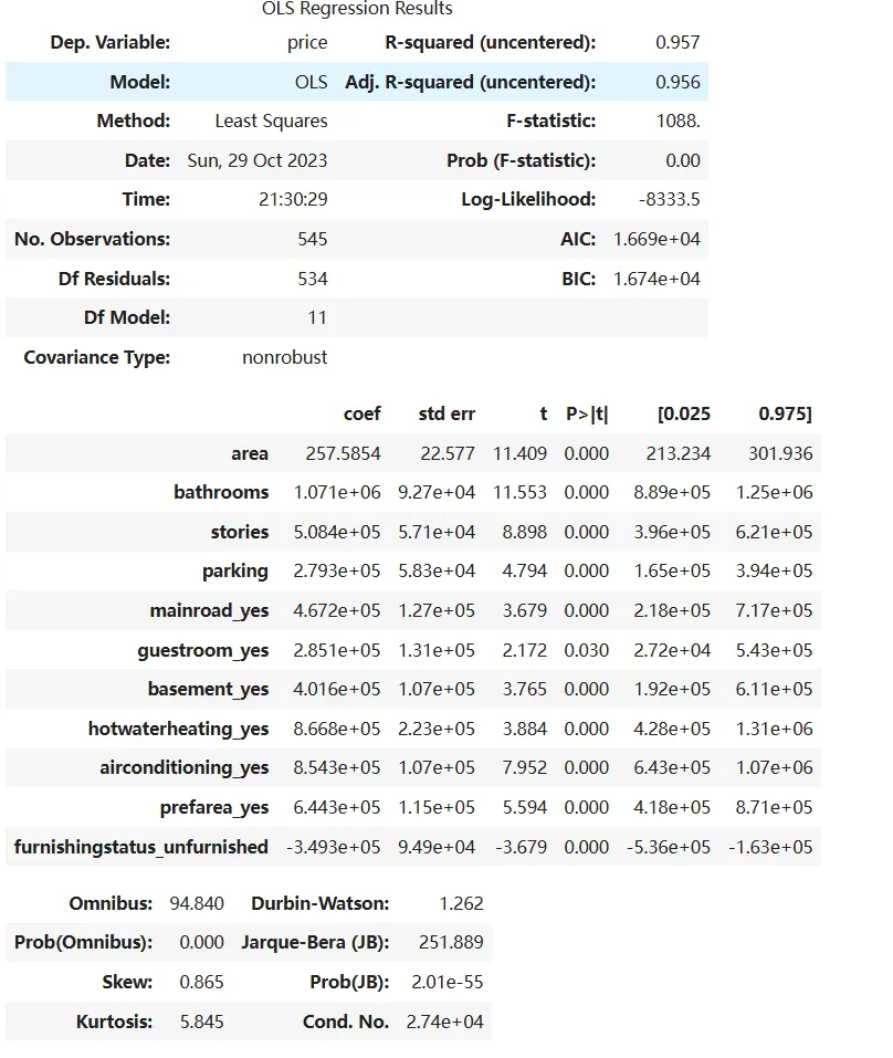
X = X.drop(['const', 'bedrooms', 'furnishingstatus_semi-furnished'], axis=1)model = sm.OLS(y, X).fit()model.summary()
新模型摘要:
- R-squared (uncentered) = 0.957,拟合度大幅提升!
- 所有剩余变量 p 值均小于 0.05,具有统计显著性。
系数解读:
- 面积、厕所数、楼层数、车库数、主路、客房、地下室、热水器、空调、首选社区都会显著提升房价。
- 毛坯房 (
furnishingstatus_unfurnished) 会显著降低房价。
🔮 预测新房屋价格
构造待预测房屋的数据(注意:目标房屋面积为 6500,但原始代码中误写为 5600,我们保留原样以便复现结果)。
price_to_predict = pd.DataFrame({'area': [5600], 'bedrooms': [4], 'bathrooms': [2],'stories': [2], 'mainroad': ['no'], 'guestroom': ['no'],'basement':['yes'], 'hotwaterheating': ['yes'],'airconditioning': ['no'], 'parking': 2, 'prefarea': ['yes'],'furnishingstatus': ['semi-furnished']})price_to_predict
将分类变量统一为 category 类型,并指定所有可能取值,确保后续的 get_dummies 不会遗漏。
price_to_predict['mainroad'] = pd.Categorical(price_to_predict['mainroad'], categories=['no', 'yes'])price_to_predict['guestroom'] = pd.Categorical(price_to_predict['guestroom'], categories=['no', 'yes'])price_to_predict['basement'] = pd.Categorical(price_to_predict['basement'], categories=['no', 'yes'])price_to_predict['hotwaterheating'] = pd.Categorical(price_to_predict['hotwaterheating'], categories=['no', 'yes'])price_to_predict['airconditioning'] = pd.Categorical(price_to_predict['airconditioning'], categories=['no', 'yes'])price_to_predict['prefarea'] = pd.Categorical(price_to_predict['prefarea'], categories=['no', 'yes'])price_to_predict['furnishingstatus'] = pd.Categorical(price_to_predict['furnishingstatus'], categories=['furnished', 'semi-furnished', 'unfurnished'])
生成虚拟变量。
price_to_predict = pd.get_dummies(price_to_predict, drop_first=True, columns=['mainroad', 'guestroom', 'basement','hotwaterheating', 'airconditioning','prefarea', 'furnishingstatus'], dtype=int)price_to_predict.head()
剔除模型中未使用的变量(卧室、简装虚拟变量)。
price_to_predict = price_to_predict.drop(['bedrooms', 'furnishingstatus_semi-furnished'], axis=1)
最后,用模型进行预测。
predicted_value = model.predict(price_to_predict)predicted_value
输出:
0 7.071927e+06dtype: float64
预测价格约为 7,071,927 元。
✅ 总结
通过本项目,我们完整走了一遍数据分析与线性回归建模的流程:
最终模型拟合度高达 95.7%,预测结果具有一定参考价值。当然,实际应用中还需考虑更多因素(如地理位置、房龄等),但本项目的思路和方法是通用的。
希望这篇推文对你有所帮助!如果你也想动手试试,可以在公众号后台回复“预测房价”获取数据集和完整代码。我们下期再见!👋

 10个月宝宝每天需要喝多少奶粉?
