简介

西太平洋副热带高压（简称西太副高）是影响东亚地区天气气候最重要的环流系统之一。它的位置、强度和形态变化，直接决定着我国夏季雨带的分布、台风的路径，甚至高温热浪的持续时间。而副高脊线，作为描述副高位置特征的关键指标，一直以来都是学者研究的重点。

在传统研究中，副高脊线的定义主要有两种思路：其一是基于位势高度场的方法——在500hPa位势高度场上，沿着副高区域（通常以5880gpm等值线为界），寻找每个经度上位势高度的最大值点，将这些点连接起来就构成了副高脊线。其二是基于风场的动力学定义，即寻找纬向风u=0且经向切变∂u/∂y>0的点。从物理意义上讲，这对应着副热带高压脊线附近从偏东风转为偏西风的关键区域，更能反映副高的动力学特征。

那么，这两种方法定义的脊线到底有多大差异？本文以2020年7月为例，将两条脊线绘制在同一张图上进行直观对比。

代码

import numpy as npimport xarray as xrimport matplotlib.pyplot as pltimport cartopy.crs as ccrsimport cartopy.feature as cfeaturefrom scipy.ndimage import gaussian_filterfrom scipy import interpolateimport pandas as pdimport warningswarnings.filterwarnings('ignore')def read_data(hgt_file_path, uwnd_file_path):"""    Read 500hPa geopotential height and u-wind data    """print("Reading data...")# Read geopotential height    ds_hgt = xr.open_dataset(hgt_file_path)    hgt_500 = ds_hgt['hgt'].sel(level=500)# Read u-wind    ds_uwnd = xr.open_dataset(uwnd_file_path)    uwnd_500 = ds_uwnd['uwnd'].sel(level=500)print(f"Data dimensions: {hgt_500.dims}")print(f"Time range: {hgt_500.time.values[0]} to {hgt_500.time.values[-1]}")print(f"Longitude range: {hgt_500.lon.values[0]:.1f}°E - {hgt_500.lon.values[-1]:.1f}°E")print(f"Latitude range: {hgt_500.lat.values[0]:.1f}°N - {hgt_500.lat.values[-1]:.1f}°N")return hgt_500, uwnd_500def calculate_hgt_ridge(hgt_data, threshold=5880, lon_range=(90, 180), lat_range=(10, 50)):"""    Calculate subtropical high ridge line based on geopotential height maximum    """    lats = hgt_data.lat.values    lons = hgt_data.lon.valuesif hasattr(hgt_data, 'values'):        hgt_values = hgt_data.valueselse:        hgt_values = hgt_data    lon_indices = np.where((lons >= lon_range[0]) & (lons <= lon_range[1]))[0]    lat_indices = np.where((lats >= lat_range[0]) & (lats <= lat_range[1]))[0]    ridge_lons = []    ridge_lats = []for i in lon_indices:        lon = lons[i]        hgt_profile = hgt_values[lat_indices, i]        profile_lats = lats[lat_indices]if np.any(hgt_profile > threshold):            max_idx = np.argmax(hgt_profile)            max_lat = profile_lats[max_idx]            max_hgt = hgt_profile[max_idx]if max_hgt > threshold:                ridge_lons.append(lon)                ridge_lats.append(max_lat)return {'lons': ridge_lons,'lats': ridge_lats    }def calculate_wind_shear_ridge(uwnd_data, hgt_data, threshold=5880, lat_range=(10, 50), lon_range=(90, 180)):"""    Calculate subtropical high ridge line based on wind shear definition:    u=0 and ∂u/∂y > 0, only within areas where hgt >= threshold    """    lats = uwnd_data.lat.values    lons = uwnd_data.lon.valuesif hasattr(uwnd_data, 'values'):        uwnd_values = uwnd_data.valueselse:        uwnd_values = uwnd_dataif hasattr(hgt_data, 'values'):        hgt_values = hgt_data.valueselse:        hgt_values = hgt_data    lon_indices = np.where((lons >= lon_range[0]) & (lons <= lon_range[1]))[0]    lat_indices = np.where((lats >= lat_range[0]) & (lats <= lat_range[1]))[0]    lats_region = lats[lat_indices]if lats_region[0] > lats_region[-1]:        lat_indices = lat_indices[::-1]        lats_region = lats[lat_indices]    ridge_lons = []    ridge_lats = []    dy = np.abs(lats_region[1] - lats_region[0]) * 111000for i in lon_indices:        lon = lons[i]        u_profile = uwnd_values[lat_indices, i]        hgt_profile = hgt_values[lat_indices, i]# Create mask for points where hgt >= threshold        hgt_mask = hgt_profile >= threshold# If no points meet the hgt threshold, skip this longitudeif not np.any(hgt_mask):continue        zero_crossings = []for j in range(len(u_profile) - 1):# Only consider points where both points are within hgt threshold regionif hgt_mask[j] and hgt_mask[j + 1]:if u_profile[j] * u_profile[j + 1] <= 0:if u_profile[j + 1] != u_profile[j]:                        lat_zero = lats_region[j] + (lats_region[j + 1] - lats_region[j]) * \                                   (0 - u_profile[j]) / (u_profile[j + 1] - u_profile[j])else:                        lat_zero = (lats_region[j] + lats_region[j + 1]) / 2                    zero_crossings.append((j, lat_zero))for j, lat_zero in zero_crossings:if j > 0 and j < len(u_profile) - 1:                du_dy = (u_profile[j + 1] - u_profile[j - 1]) / (2 * dy)elif j == 0:                du_dy = (u_profile[1] - u_profile[0]) / dyelse:                du_dy = (u_profile[-1] - u_profile[-2]) / dyif du_dy > 0:                ridge_lons.append(lon)                ridge_lats.append(lat_zero)breakreturn {'lons': ridge_lons,'lats': ridge_lats    }def smooth_line(lons, lats, sigma=1.0):"""    Smooth ridge line using Gaussian filter    """if len(lons) < 3:return lons, lats    lats_array = np.array(lats)    lats_smooth = gaussian_filter(lats_array, sigma=sigma)return lons, lats_smooth.tolist()def plot_dual_ridges(hgt_data, uwnd_data, hgt_ridge, wind_ridge,                     year=1979, month=7, threshold=5880):"""    Plot subtropical high with both HGT-defined and wind-defined ridge lines    """    fig = plt.figure(figsize=(15, 9))    ax = plt.axes(projection=ccrs.PlateCarree(central_longitude=180))# Set map extent (western Pacific region)    ax.set_extent([100, 170, 5, 45], crs=ccrs.PlateCarree())# Add map features    ax.add_feature(cfeature.COASTLINE, linewidth=0.8)    ax.add_feature(cfeature.LAND, color='lightgray', alpha=0.5)    ax.add_feature(cfeature.OCEAN, color='lightblue', alpha=0.3)# Add gridlines    gl = ax.gridlines(draw_labels=True, linewidth=0.5, color='gray', alpha=0.5)    gl.top_labels = False    gl.right_labels = False# Prepare geopotential height dataif hasattr(hgt_data, 'values'):        hgt_values = hgt_data.values        lons = hgt_data.lon.values        lats = hgt_data.lat.valueselse:        hgt_values = hgt_data        lons = hgt_data.lon.values        lats = hgt_data.lat.values# Limit plotting region    lon_mask = (lons >= 80) & (lons <= 180)    lat_mask = (lats >= 0) & (lats <= 60)    lons_plot = lons[lon_mask]    lats_plot = lats[lat_mask]    hgt_plot = hgt_values[np.ix_(lat_mask, lon_mask)]# Create meshgrid    lons_2d, lats_2d = np.meshgrid(lons_plot, lats_plot)# Fill levels for contourf    fill_levels = np.arange(threshold - 1, 6000, 10)# Plot subtropical high area (geopotential height >= threshold)    cf = ax.contourf(lons_2d, lats_2d, hgt_plot,                     levels=fill_levels,                     cmap='YlOrRd',                     transform=ccrs.PlateCarree(),                     alpha=0.7,                     extend='max')# Plot threshold line    cs = ax.contour(lons_2d, lats_2d, hgt_plot,                    levels=[threshold],                    colors='r',                    linewidths=2,                    transform=ccrs.PlateCarree())    ax.clabel(cs, inline=True, fontsize=9, fmt='%d')# Add colorbar    plt.colorbar(cf, ax=ax, label=f'Geopotential height (gpm)',                 shrink=0.8, pad=0.05)# Plot HGT-defined ridge line (in blue)if len(hgt_ridge['lons']) > 0:        lons_smooth, lats_smooth = smooth_line(hgt_ridge['lons'], hgt_ridge['lats'], sigma=1.0)        ax.plot(lons_smooth, lats_smooth, 'b-', linewidth=4.5,                transform=ccrs.PlateCarree(),                label='HGT-defined ridge (max HGT)',                zorder=10)        ax.scatter(hgt_ridge['lons'], hgt_ridge['lats'],                   c='blue', s=30, transform=ccrs.PlateCarree(),                   zorder=11, edgecolors='white', linewidth=0.5, alpha=0.7)# Plot wind-defined ridge line (in green)if len(wind_ridge['lons']) > 0:        lons_smooth, lats_smooth = smooth_line(wind_ridge['lons'], wind_ridge['lats'], sigma=1.0)        ax.plot(lons_smooth, lats_smooth, 'g-', linewidth=4,                transform=ccrs.PlateCarree(),                label='Wind-defined ridge (u=0, ∂u/∂y>0, within HGT≥5880)',                zorder=10)        ax.scatter(wind_ridge['lons'], wind_ridge['lats'],                   c='green', s=30, transform=ccrs.PlateCarree(),                   zorder=11, edgecolors='white', linewidth=0.5, alpha=0.7)# Add legend    plt.legend(loc='upper right', fontsize=11)# Add longitude labelsfor lon in [110, 120, 130, 140, 150, 160]:        ax.axvline(x=lon, color='gray', linestyle='--', linewidth=0.5, alpha=0.3)        ax.text(lon, 6, f'{lon}°E', transform=ccrs.PlateCarree(),                ha='center', fontsize=8, color='gray')# Add latitude labelsfor lat in [10, 20, 30, 40]:        ax.axhline(y=lat, color='gray', linestyle='--', linewidth=0.5, alpha=0.3)        ax.text(102, lat, f'{lat}°N', transform=ccrs.PlateCarree(),                va='center', fontsize=8, color='gray')    plt.tight_layout()# Save figure    output_file = f'wpsh_dual_ridges_{year}_{month:02d}.png'    plt.savefig(output_file, dpi=300, bbox_inches='tight')print(f"Figure saved to: {output_file}")    plt.show()return fig, axdef main():"""    Main function: Calculate and plot both HGT-defined and wind-defined ridge lines    """# Data file paths    hgt_file_path = "hgt.mon.mean.nc"    uwnd_file_path = "uwnd.mon.mean.nc"# Read data    try:        hgt_500, uwnd_500 = read_data(hgt_file_path, uwnd_file_path)    except FileNotFoundError as e:print(f"Error: File not found - {e}")print("Please ensure both hgt.mon.mean.nc and uwnd.mon.mean.nc files are in the current directory")return    except Exception as e:print(f"Error reading data: {e}")return# User input for year and monthprint("\n" + "=" * 50)print("Select year and month for analysis")    years = pd.to_datetime(hgt_500.time.values).year    unique_years = sorted(set(years))print(f"Available years: {min(unique_years)} - {max(unique_years)}")    try:        year = int(input("Enter year (e.g., 2020): "))        month = int(input("Enter month (1-12): "))if month < 1 or month > 12:print("Month must be between 1-12")return    except ValueError:print("Please enter valid numbers")return# Find data for specified year and monthprint(f"\nSearching for {year}/{month:02d} data...")    time_array = pd.to_datetime(hgt_500.time.values)    mask = (time_array.year == year) & (time_array.month == month)    matching_indices = np.where(mask)[0]if len(matching_indices) == 0:print(f"Error: No data found for {year}/{month:02d}")print(f"Available years: {min(unique_years)}-{max(unique_years)}")return    idx = matching_indices[0]    target_time = hgt_500.time.values[idx]    target_hgt = hgt_500.isel(time=idx)    target_uwnd = uwnd_500.isel(time=idx)print(f"Found data: {pd.to_datetime(target_time).strftime('%Y-%m')}")# Set subtropical high threshold    threshold = 5880# Calculate HGT-defined ridge lineprint("\nCalculating HGT-defined ridge line (based on geopotential height maximum)...")    hgt_ridge = calculate_hgt_ridge(target_hgt, threshold,                                    lon_range=(90, 180),                                    lat_range=(10, 50))# Calculate wind-defined ridge line (only within HGT≥5880 area)print("Calculating wind-defined ridge line (based on u=0 and ∂u/∂y>0, only within HGT≥5880 area)...")    wind_ridge = calculate_wind_shear_ridge(target_uwnd, target_hgt, threshold,                                            lon_range=(90, 180),                                            lat_range=(10, 50))# Plot both ridge linesprint("\nPlotting both ridge lines for comparison...")    plot_dual_ridges(target_hgt, target_uwnd, hgt_ridge, wind_ridge,                     year, month, threshold)print("\nDone!")if __name__ == "__main__":    main()

结果

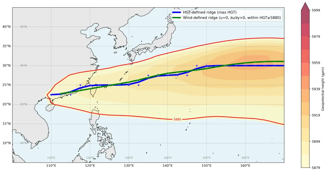结果显示，两者差别不大，看起来基于风场的结果更平滑，这可能是数据分辨率和基于风场的计算方法综合影响的结果，例如线性插值与梯度计算的平滑作用。