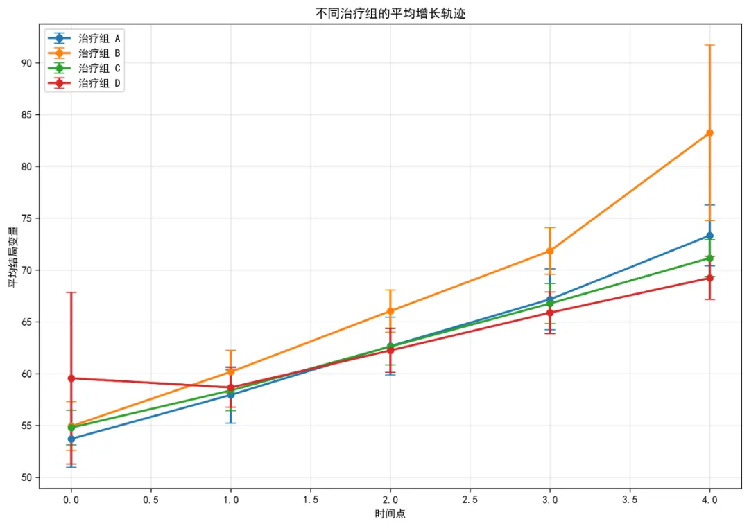
# pip install pandas numpy matplotlib seaborn scipy statsmodels scikit-learn python-docximport osimport warningsimport numpy as npimport pandas as pdimport matplotlib.pyplot as pltimport seaborn as snsfrom scipy import statsfrom scipy.optimize import curve_fitimport statsmodels.api as smimport statsmodels.formula.api as smffrom statsmodels.tools.tools import add_constantfrom sklearn.preprocessing import StandardScalerfrom datetime import datetimeimport jsonfrom pathlib import Pathfrom docx import Documentfrom docx.shared import Inchesfrom docx.enum.text import WD_ALIGN_PARAGRAPHfrom docx.enum.table import WD_TABLE_ALIGNMENTimport matplotlibmatplotlib.use('Agg') # 非交互式后端# 设置中文显示plt.rcParams['font.sans-serif'] = ['SimHei', 'DejaVu Sans']plt.rcParams['axes.unicode_minus'] = False# 忽略警告warnings.filterwarnings('ignore')# ==============================# 0. 设置工作目录和结果文件夹# ==============================# 自动寻找桌面路径desktop_path = Path.home() / 'Desktop'os.chdir(desktop_path)# 创建结果文件夹results_dir = desktop_path / '10-NLME结果'results_dir.mkdir(exist_ok=True)os.chdir(results_dir)# ==============================# 1. 数据读取与预处理# ==============================print("1. 数据读取与预处理...")# 读取Excel数据try: data_file = desktop_path / 'longitudinal_data.xlsx' simple_data = pd.read_excel(data_file, sheet_name='Simple_Dataset')except FileNotFoundError:print(f"错误: 未找到文件 {data_file}")print("创建示例数据以供演示...")# 创建示例数据 np.random.seed(123) n_subjects = 100 n_timepoints = 5 subjects = []times = [] outcomes = [] treatments = [] ages = [] baselines = [] sexes = [] schools = [] dates = [] treatments_list = ['A', 'B', 'C', 'D']for i in range(n_subjects): subject_id = f"SUB{i + 1:03d}" treatment = np.random.choice(treatments_list) age = np.random.normal(45, 10) baseline = np.random.normal(50, 10) sex = np.random.choice(['M', 'F']) school = f"SCH{np.random.randint(1, 6)}"# 指数增长轨迹 time_points = np.arange(n_timepoints) base_outcome = baseline * np.exp(0.05 * time_points)# 添加随机效应 random_effect = np.random.normal(0, 5)# 添加治疗效应if treatment == 'B': treatment_effect = 5elif treatment == 'C': treatment_effect = 10elif treatment == 'D': treatment_effect = 15else: treatment_effect = 0 outcome = base_outcome + random_effect + treatment_effect + np.random.normal(0, 2, n_timepoints)# 添加到列表 subjects.extend([subject_id] * n_timepoints) times.extend(time_points) outcomes.extend(outcome) treatments.extend([treatment] * n_timepoints) ages.extend([age] * n_timepoints) baselines.extend([baseline] * n_timepoints) sexes.extend([sex] * n_timepoints) schools.extend([school] * n_timepoints) dates.extend([datetime(2023, 1, 1) + pd.Timedelta(days=t * 30) for t in time_points]) simple_data = pd.DataFrame({'ID': subjects,'Time': times,'Outcome': outcomes,'Treatment': treatments,'Age': ages,'Baseline_Score': baselines,'Sex': sexes,'School_ID': schools,'Measurement_Date': dates })# 保存示例数据 simple_data.to_excel(data_file, sheet_name='Simple_Dataset', index=False)print(f"已创建示例数据并保存到: {data_file}")# 数据清洗和转换simple_data['ID'] = simple_data['ID'].astype('category')simple_data['Time'] = pd.to_numeric(simple_data['Time'], errors='coerce')simple_data['Age'] = pd.to_numeric(simple_data['Age'], errors='coerce')simple_data['Sex'] = simple_data['Sex'].astype('category')simple_data['Treatment'] = simple_data['Treatment'].astype('category')simple_data['Baseline_Score'] = pd.to_numeric(simple_data['Baseline_Score'], errors='coerce')simple_data['School_ID'] = simple_data['School_ID'].astype('category')if'Measurement_Date'in simple_data.columns: simple_data['Measurement_Date'] = pd.to_datetime(simple_data['Measurement_Date'], errors='coerce')simple_data['Outcome'] = pd.to_numeric(simple_data['Outcome'], errors='coerce')# 删除完全缺失Outcome的行simple_data = simple_data.dropna(subset=['Outcome'])# 查看数据结构print("\n数据集结构:")print(f"行数: {simple_data.shape[0]}, 列数: {simple_data.shape[1]}")print("\n数据摘要:")print(simple_data.describe())print("\n数据类型:")print(simple_data.dtypes)# 保存清洗后的数据simple_data.to_csv('清洗后数据.csv', index=False, encoding='utf-8-sig')# ==============================# 2. 探索性数据分析# ==============================print("\n2. 探索性数据分析...")# 创建图形文件夹fig_dir = results_dir / 'figures'fig_dir.mkdir(exist_ok=True)# 2.1 个体增长轨迹plt.figure(figsize=(12, 8))for subject_id in simple_data['ID'].unique()[:50]: # 只显示前50个个体避免过度拥挤 subject_data = simple_data[simple_data['ID'] == subject_id] plt.plot(subject_data['Time'], subject_data['Outcome'], color='gray', alpha=0.3, linewidth=0.5)# 添加平滑曲线from scipy.interpolate import make_interp_splinetry: time_sorted = simple_data['Time'].sort_values().unique() mean_outcome_by_time = simple_data.groupby('Time')['Outcome'].mean().reindex(time_sorted)# 使用样条插值获得平滑曲线if len(time_sorted) > 3: x_smooth = np.linspace(time_sorted.min(), time_sorted.max(), 300) spl = make_interp_spline(time_sorted, mean_outcome_by_time.values, k=3) y_smooth = spl(x_smooth) plt.plot(x_smooth, y_smooth, color='red', linewidth=2, label='平均趋势')except Exception as e:print(f"平滑曲线绘制失败: {e}")plt.scatter(simple_data['Time'], simple_data['Outcome'], alpha=0.2, s=10, color='blue')plt.title('个体增长轨迹图')plt.xlabel('时间点')plt.ylabel('结局变量')plt.grid(True, alpha=0.3)plt.savefig(fig_dir / '01_个体增长轨迹.png', dpi=300, bbox_inches='tight')plt.close()# 2.2 按治疗组分组的平均轨迹plt.figure(figsize=(12, 8))for treatment in simple_data['Treatment'].cat.categories: treatment_data = simple_data[simple_data['Treatment'] == treatment] mean_by_time = treatment_data.groupby('Time')['Outcome'].agg(['mean', 'std', 'count']) mean_by_time['se'] = mean_by_time['std'] / np.sqrt(mean_by_time['count']) plt.errorbar(mean_by_time.index, mean_by_time['mean'], yerr=1.96 * mean_by_time['se'], label=f'治疗组 {treatment}', capsize=5, linewidth=2, marker='o')plt.title('不同治疗组的平均增长轨迹')plt.xlabel('时间点')plt.ylabel('平均结局变量')plt.legend()plt.grid(True, alpha=0.3)plt.savefig(fig_dir / '02_治疗组平均轨迹.png', dpi=300, bbox_inches='tight')plt.close()

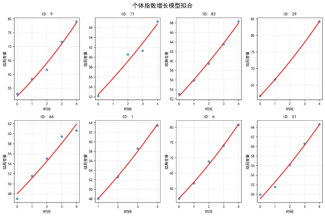
if len(individual_stats_df) > 0: plt.figure(figsize=(10, 8)) plt.scatter(individual_stats_df['Intercept'], individual_stats_df['Slope'], alpha=0.6, s=50)# 添加回归线if len(individual_stats_df) > 1: from scipy.stats import linregress slope, intercept, r_value, p_value, std_err = linregress( individual_stats_df['Intercept'], individual_stats_df['Slope'] ) x_range = np.array([individual_stats_df['Intercept'].min(), individual_stats_df['Intercept'].max()]) plt.plot(x_range, intercept + slope * x_range, color='red', linewidth=2, label=f'回归线 (r={r_value:.3f})') plt.legend() plt.title('个体截距与斜率的关系') plt.xlabel('截距(初始值)') plt.ylabel('斜率(增长速率)') plt.grid(True, alpha=0.3) plt.savefig(fig_dir / '03_截距斜率关系.png', dpi=300, bbox_inches='tight') plt.close()# 2.4 创建合并图fig, axes = plt.subplots(2, 2, figsize=(16, 12))# 子图1: 个体增长轨迹(简化版)for subject_id in simple_data['ID'].unique()[:30]: # 只显示前30个 subject_data = simple_data[simple_data['ID'] == subject_id] axes[0, 0].plot(subject_data['Time'], subject_data['Outcome'], color='gray', alpha=0.3, linewidth=0.5)axes[0, 0].scatter(simple_data['Time'], simple_data['Outcome'], alpha=0.1, s=5, color='blue')axes[0, 0].set_title('个体增长轨迹图')axes[0, 0].set_xlabel('时间点')axes[0, 0].set_ylabel('结局变量')axes[0, 0].grid(True, alpha=0.3)# 子图2: 治疗组平均轨迹for treatment in simple_data['Treatment'].cat.categories: treatment_data = simple_data[simple_data['Treatment'] == treatment] mean_by_time = treatment_data.groupby('Time')['Outcome'].mean() axes[0, 1].plot(mean_by_time.index, mean_by_time.values, label=f'治疗组 {treatment}', linewidth=2, marker='o')axes[0, 1].set_title('不同治疗组的平均增长轨迹')axes[0, 1].set_xlabel('时间点')axes[0, 1].set_ylabel('平均结局变量')axes[0, 1].legend()axes[0, 1].grid(True, alpha=0.3)# 子图3: 截距斜率关系if len(individual_stats_df) > 0: axes[1, 0].scatter(individual_stats_df['Intercept'], individual_stats_df['Slope'], alpha=0.6, s=50) axes[1, 0].set_title('个体截距与斜率的关系') axes[1, 0].set_xlabel('截距(初始值)') axes[1, 0].set_ylabel('斜率(增长速率)') axes[1, 0].grid(True, alpha=0.3)# 子图4: 数据分布axes[1, 1].hist(simple_data['Outcome'], bins=30, edgecolor='black', alpha=0.7)axes[1, 1].set_title('结局变量分布')axes[1, 1].set_xlabel('结局变量值')axes[1, 1].set_ylabel('频数')axes[1, 1].grid(True, alpha=0.3)plt.tight_layout()plt.savefig(fig_dir / '04_探索性数据分析合并图.png', dpi=300, bbox_inches='tight')plt.close()# ==============================# 3. 非线性混合效应模型准备# ==============================print("\n3. 准备非线性混合效应模型数据...")# 复制数据并创建新变量nlme_data = simple_data.copy()# 标准化连续变量scaler_age = StandardScaler()scaler_baseline = StandardScaler()nlme_data['Age_c'] = scaler_age.fit_transform(nlme_data[['Age']])nlme_data['Baseline_c'] = scaler_baseline.fit_transform(nlme_data[['Baseline_Score']])# 确保Treatment是分类变量并设置参考水平nlme_data['Treatment'] = pd.Categorical(nlme_data['Treatment'])nlme_data['Treatment'] = nlme_data['Treatment'].cat.reorder_categories( sorted(nlme_data['Treatment'].cat.categories))# ==============================# 4. 指数增长模型拟合# ==============================print("\n4. 拟合指数增长模型...")def exponential_func(t, A, B):"""指数函数: y = A * exp(B * t)"""return A * np.exp(B * t)# 首先为每个个体拟合单独的指数模型,获取初始参数估计individual_params = []valid_subjects = []for subject_id in nlme_data['ID'].unique(): subject_data = nlme_data[nlme_data['ID'] == subject_id]if len(subject_data) >= 3: # 需要足够的数据点 try:# 初始参数估计 A_init = subject_data['Outcome'].iloc[0] B_init = 0.05# 拟合曲线 params, _ = curve_fit(exponential_func, subject_data['Time'], subject_data['Outcome'], p0=[A_init, B_init], maxfev=10000) individual_params.append({'ID': subject_id,'A': params[0],'B': params[1] }) valid_subjects.append(subject_id) except:continueif len(individual_params) > 0: param_df = pd.DataFrame(individual_params)print(f"成功拟合 {len(param_df)} 个个体的指数模型")# 使用平均参数作为整体模型的初始值 A_init_global = param_df['A'].median() B_init_global = param_df['B'].median()print(f"全局初始参数: A={A_init_global:.2f}, B={B_init_global:.4f}")# 保存个体参数 param_df.to_csv('指数模型个体参数.csv', index=False, encoding='utf-8-sig')# 可视化个体拟合 plt.figure(figsize=(12, 8))# 随机选择几个个体显示 np.random.seed(123) sample_ids = np.random.choice(valid_subjects, min(8, len(valid_subjects)), replace=False)for i, subject_id in enumerate(sample_ids): subject_data = nlme_data[nlme_data['ID'] == subject_id] subject_param = param_df[param_df['ID'] == subject_id].iloc[0]# 生成平滑曲线 t_smooth = np.linspace(subject_data['Time'].min(), subject_data['Time'].max(), 100) y_smooth = exponential_func(t_smooth, subject_param['A'], subject_param['B']) plt.subplot(2, 4, i + 1) plt.scatter(subject_data['Time'], subject_data['Outcome'], alpha=0.7, s=30) plt.plot(t_smooth, y_smooth, 'r-', linewidth=2) plt.title(f'ID: {subject_id}') plt.xlabel('时间') plt.ylabel('结局变量') plt.grid(True, alpha=0.3) plt.suptitle('个体指数增长模型拟合', fontsize=16) plt.tight_layout() plt.savefig(fig_dir / '05_个体指数模型拟合.png', dpi=300, bbox_inches='tight') plt.close()# 整体数据拟合(不考虑随机效应) try: all_times = nlme_data['Time'].values all_outcomes = nlme_data['Outcome'].values popt, pcov = curve_fit(exponential_func, all_times, all_outcomes, p0=[A_init_global, B_init_global], maxfev=10000)print(f"整体指数模型参数: A={popt[0]:.2f}, B={popt[1]:.4f}")# 可视化整体拟合 plt.figure(figsize=(10, 6)) plt.scatter(all_times, all_outcomes, alpha=0.1, s=10, label='原始数据') t_smooth = np.linspace(all_times.min(), all_times.max(), 100) y_smooth = exponential_func(t_smooth, popt[0], popt[1]) plt.plot(t_smooth, y_smooth, 'r-', linewidth=3, label='指数拟合') plt.title('整体指数增长模型拟合') plt.xlabel('时间') plt.ylabel('结局变量') plt.legend() plt.grid(True, alpha=0.3) plt.savefig(fig_dir / '06_整体指数模型拟合.png', dpi=300, bbox_inches='tight') plt.close() exp_model_success = True exp_params = popt except Exception as e:print(f"整体指数模型拟合失败: {e}") exp_model_success = False exp_params = Noneelse:print("没有足够的个体数据拟合指数模型") exp_model_success = False exp_params = None# ==============================# 5. 逻辑斯蒂增长模型拟合# ==============================print("\n5. 拟合逻辑斯蒂增长模型...")def logistic_func(t, Asym, xmid, scal):"""逻辑斯蒂函数: y = Asym / (1 + exp((xmid - t)/scal))"""return Asym / (1 + np.exp((xmid - t) / scal))# 尝试拟合逻辑斯蒂模型try:# 获取合理初始值 Asym_init = nlme_data['Outcome'].max() * 1.1 # 渐近线略大于最大值 xmid_init = nlme_data['Time'].median() # 中点在中位数时间 scal_init = 1.0 # 尺度参数# 使用curve_fit拟合 popt_logistic, pcov_logistic = curve_fit(logistic_func, nlme_data['Time'].values, nlme_data['Outcome'].values, p0=[Asym_init, xmid_init, scal_init], maxfev=10000)print(f"逻辑斯蒂模型参数: Asym={popt_logistic[0]:.2f}, " f"xmid={popt_logistic[1]:.2f}, scal={popt_logistic[2]:.2f}")# 可视化逻辑斯蒂拟合 plt.figure(figsize=(10, 6)) plt.scatter(nlme_data['Time'], nlme_data['Outcome'], alpha=0.1, s=10, label='原始数据') t_smooth = np.linspace(nlme_data['Time'].min(), nlme_data['Time'].max(), 100) y_smooth = logistic_func(t_smooth, *popt_logistic) plt.plot(t_smooth, y_smooth, 'g-', linewidth=3, label='逻辑斯蒂拟合') plt.title('逻辑斯蒂增长模型拟合') plt.xlabel('时间') plt.ylabel('结局变量') plt.legend() plt.grid(True, alpha=0.3) plt.savefig(fig_dir / '07_逻辑斯蒂模型拟合.png', dpi=300, bbox_inches='tight') plt.close() logistic_model_success = True logistic_params = popt_logisticexcept Exception as e:print(f"逻辑斯蒂模型拟合失败: {e}") logistic_model_success = False logistic_params = None# ==============================# 6. 线性混合模型(二次增长模型)# ==============================print("\n6. 拟合线性混合模型(二次增长模型)...")# 准备数据mixed_data = nlme_data.copy()# 创建时间平方项mixed_data['Time_sq'] = mixed_data['Time'] ** 2# 创建虚拟变量(用于Treatment)mixed_data = pd.get_dummies(mixed_data, columns=['Treatment'], prefix='Treatment', drop_first=False)# 提取treatment列名treatment_cols = [col for col in mixed_data.columns if col.startswith('Treatment_')]# 构建混合模型公式# 基础固定效应base_formula = 'Outcome ~ Time + Time_sq + Age_c + Baseline_c'# 添加治疗组效应(避免虚拟变量陷阱)if len(treatment_cols) > 1:# 使用所有treatment列,但模型会自动处理多重共线性 treatment_formula = ' + '.join(treatment_cols) formula = f'{base_formula} + {treatment_formula}'else: formula = base_formula# 添加随机效应(随机截距和随机斜率)formula_with_random = f'{formula} + (1 + Time | ID)'print(f"模型公式: {formula_with_random}")try:# 使用statsmodels的MixedLM# 注意:statsmodels的MixedLM不支持复杂的随机效应结构如(1 + Time | ID)# 这里我们简化,只使用随机截距# 简化公式:只有随机截距 formula_simple = f'{formula}'# 为MixedLM准备数据# 我们需要为随机效应创建组变量 mixed_data['group'] = mixed_data['ID']# 拟合混合模型 from statsmodels.regression.mixed_linear_model import MixedLM# 准备设计矩阵 X = pd.get_dummies(mixed_data[['Time', 'Time_sq', 'Age_c', 'Baseline_c'] + treatment_cols], drop_first=True) X = sm.add_constant(X) y = mixed_data['Outcome'] groups = mixed_data['group']# 拟合模型 mixed_model = MixedLM(y, X, groups) mixed_result = mixed_model.fit()print("混合模型拟合成功!")print(mixed_result.summary())# 提取固定效应 fixed_effects = mixed_result.params fixed_se = mixed_result.bse# 计算t值和p值 t_values = fixed_effects / fixed_se p_values = 2 * (1 - stats.t.cdf(np.abs(t_values), mixed_result.df_resid))# 创建固定效应表 fixed_table = pd.DataFrame({'参数': fixed_effects.index,'估计值': fixed_effects.values,'标准误': fixed_se.values,'t值': t_values.values,'p值': p_values.values })# 添加显著性标记 conditions = [ fixed_table['p值'] < 0.001, fixed_table['p值'] < 0.01, fixed_table['p值'] < 0.05 ] choices = ['***', '**', '*'] fixed_table['显著性'] = np.select(conditions, choices, default='')# 保存固定效应表 fixed_table.to_csv('08_混合模型固定效应.csv', index=False, encoding='utf-8-sig')# 提取随机效应 random_effects = mixed_result.random_effects random_df = pd.DataFrame()for group, effects in random_effects.items(): temp_df = pd.DataFrame(effects, index=[group]) random_df = pd.concat([random_df, temp_df]) random_df.columns = ['随机截距'] random_df.to_csv('09_混合模型随机效应.csv', encoding='utf-8-sig')# 计算组内相关系数(ICC)# ICC = 组间方差 / (组间方差 + 组内方差) try:# 提取方差成分 vc = mixed_result.cov_re.iloc[0, 0] # 随机截距方差 residual_var = mixed_result.scale # 残差方差 total_var = vc + residual_var icc = vc / total_varprint(f"随机截距方差: {vc:.4f}")print(f"残差方差: {residual_var:.4f}")print(f"组内相关系数(ICC): {icc:.4f} ({icc * 100:.1f}%)") except: icc = None quadratic_model_success = True quadratic_model = mixed_resultexcept Exception as e:print(f"混合模型拟合失败: {e}") import traceback traceback.print_exc() quadratic_model_success = False quadratic_model = None# ==============================# 7. 模型比较# ==============================print("\n7. 模型比较...")model_comparison = []# 指数模型比较if exp_model_success and exp_params is not None:# 计算指数模型的拟合优度 y_true = nlme_data['Outcome'].values y_pred_exp = exponential_func(nlme_data['Time'].values, exp_params[0], exp_params[1])# 计算残差平方和 rss_exp = np.sum((y_true - y_pred_exp) ** 2) tss = np.sum((y_true - np.mean(y_true)) ** 2) r_squared_exp = 1 - (rss_exp / tss)# 计算AIC和BIC(近似) n_params_exp = 2 # A, B两个参数 n_obs = len(y_true) aic_exp = n_obs * np.log(rss_exp / n_obs) + 2 * n_params_exp bic_exp = n_obs * np.log(rss_exp / n_obs) + n_params_exp * np.log(n_obs) model_comparison.append({'模型': '指数增长模型','AIC': round(aic_exp, 2),'BIC': round(bic_exp, 2),'R²': round(r_squared_exp, 4),'参数个数': n_params_exp })# 逻辑斯蒂模型比较if logistic_model_success and logistic_params is not None: y_true = nlme_data['Outcome'].values y_pred_logistic = logistic_func(nlme_data['Time'].values, *logistic_params) rss_logistic = np.sum((y_true - y_pred_logistic) ** 2) r_squared_logistic = 1 - (rss_logistic / tss) n_params_logistic = 3 # Asym, xmid, scal aic_logistic = n_obs * np.log(rss_logistic / n_obs) + 2 * n_params_logistic bic_logistic = n_obs * np.log(rss_logistic / n_obs) + n_params_logistic * np.log(n_obs) model_comparison.append({'模型': '逻辑斯蒂模型','AIC': round(aic_logistic, 2),'BIC': round(bic_logistic, 2),'R²': round(r_squared_logistic, 4),'参数个数': n_params_logistic })# 混合模型比较if quadratic_model_success and quadratic_model is not None:# 使用模型自带的AIC和BIC aic_mixed = quadratic_model.aic bic_mixed = quadratic_model.bic# 计算R² y_pred_mixed = quadratic_model.fittedvalues rss_mixed = np.sum((mixed_data['Outcome'] - y_pred_mixed) ** 2) r_squared_mixed = 1 - (rss_mixed / tss) n_params_mixed = len(quadratic_model.params) + 1 # 固定效应 + 随机效应方差 model_comparison.append({'模型': '混合效应模型','AIC': round(aic_mixed, 2),'BIC': round(bic_mixed, 2),'R²': round(r_squared_mixed, 4),'参数个数': n_params_mixed })# 创建比较表if model_comparison: comparison_df = pd.DataFrame(model_comparison) comparison_df = comparison_df.sort_values('AIC') comparison_df.to_csv('10_模型比较.csv', index=False, encoding='utf-8-sig')print("\n模型比较结果:")print(comparison_df.to_string(index=False))# 选择最佳模型 best_model_name = comparison_df.iloc[0]['模型']print(f"\n最佳模型: {best_model_name} (AIC最低)")# 根据模型名称分配最佳模型if best_model_name == '指数增长模型': best_model = {'type': 'exponential', 'params': exp_params}elif best_model_name == '逻辑斯蒂模型': best_model = {'type': 'logistic', 'params': logistic_params}else: best_model = {'type': 'mixed', 'model': quadratic_model}else:print("没有可比较的模型") best_model = None best_model_name = "无"# ==============================# 8. 模型可视化# ==============================print("\n8. 模型可视化...")if best_model is not None:# 8.1 总体拟合曲线 plt.figure(figsize=(12, 8))# 绘制原始数据点for treatment in nlme_data['Treatment'].cat.categories: treatment_data = nlme_data[nlme_data['Treatment'] == treatment] plt.scatter(treatment_data['Time'], treatment_data['Outcome'], alpha=0.3, s=20, label=f'治疗组 {treatment}')# 根据模型类型绘制拟合曲线 time_range = np.linspace(nlme_data['Time'].min(), nlme_data['Time'].max(), 100)if best_model['type'] == 'exponential': y_fit = exponential_func(time_range, best_model['params'][0], best_model['params'][1]) plt.plot(time_range, y_fit, 'k-', linewidth=3, label='指数模型拟合')elif best_model['type'] == 'logistic': y_fit = logistic_func(time_range, *best_model['params']) plt.plot(time_range, y_fit, 'k-', linewidth=3, label='逻辑斯蒂模型拟合')elif best_model['type'] == 'mixed':# 为混合模型创建预测数据# 这里简化,使用平均协变量值 pred_data = pd.DataFrame({'Time': time_range,'Time_sq': time_range ** 2,'Age_c': 0,'Baseline_c': 0 })# 添加treatment列(使用参考组)for col in treatment_cols: pred_data[col] = 0if'Treatment_A'in pred_data.columns: pred_data['Treatment_A'] = 1# 添加常数项 pred_data['const'] = 1# 确保列顺序与模型一致 X_pred = pred_data[quadratic_model.params.index]# 预测 y_fit = quadratic_model.predict(X_pred) plt.plot(time_range, y_fit, 'k-', linewidth=3, label='混合模型拟合') plt.title(f'最佳模型拟合曲线 - {best_model_name}') plt.xlabel('时间点') plt.ylabel('结局变量') plt.legend() plt.grid(True, alpha=0.3) plt.savefig(fig_dir / '11_最佳模型拟合曲线.png', dpi=300, bbox_inches='tight') plt.close()# 8.2 个体预测曲线(随机选择8个个体) np.random.seed(123) sample_ids = np.random.choice(nlme_data['ID'].unique(), min(8, len(nlme_data['ID'].unique())), replace=False) fig, axes = plt.subplots(2, 4, figsize=(16, 10)) axes = axes.flatten()for i, subject_id in enumerate(sample_ids):if i >= len(axes):break subject_data = nlme_data[nlme_data['ID'] == subject_id]# 绘制个体数据点 axes[i].scatter(subject_data['Time'], subject_data['Outcome'], alpha=0.7, s=50)# 个体线性拟合(二次多项式)if len(subject_data) >= 3: try:# 二次多项式拟合 coeffs = np.polyfit(subject_data['Time'], subject_data['Outcome'], 2) poly_func = np.poly1d(coeffs) t_smooth = np.linspace(subject_data['Time'].min(), subject_data['Time'].max(), 50) y_smooth = poly_func(t_smooth) axes[i].plot(t_smooth, y_smooth, 'r-', linewidth=2) except: pass axes[i].set_title(f'ID: {subject_id}') axes[i].set_xlabel('时间点') axes[i].set_ylabel('结局变量') axes[i].grid(True, alpha=0.3) plt.suptitle('个体增长曲线 (随机选择8个个体)', fontsize=16) plt.tight_layout() plt.savefig(fig_dir / '12_个体增长曲线.png', dpi=300, bbox_inches='tight') plt.close()# 8.3 模型诊断图(针对混合模型)if best_model['type'] == 'mixed' and quadratic_model_success:# 残差分析 residuals = quadratic_model.resid fitted_values = quadratic_model.fittedvalues fig, axes = plt.subplots(2, 3, figsize=(15, 10))# 1. 残差与拟合值图 axes[0, 0].scatter(fitted_values, residuals, alpha=0.5) axes[0, 0].axhline(y=0, color='r', linestyle='--') axes[0, 0].set_xlabel('拟合值') axes[0, 0].set_ylabel('残差') axes[0, 0].set_title('残差图') axes[0, 0].grid(True, alpha=0.3)# 2. Q-Q图 stats.probplot(residuals, dist="norm", plot=axes[0, 1]) axes[0, 1].set_title('Q-Q图') axes[0, 1].grid(True, alpha=0.3)# 3. 残差直方图 axes[0, 2].hist(residuals, bins=30, edgecolor='black', alpha=0.7) axes[0, 2].set_xlabel('残差') axes[0, 2].set_ylabel('频数') axes[0, 2].set_title('残差分布') axes[0, 2].grid(True, alpha=0.3)# 4. 残差序列图 axes[1, 0].plot(residuals, 'b-', alpha=0.7) axes[1, 0].axhline(y=0, color='r', linestyle='--') axes[1, 0].set_xlabel('观察序号') axes[1, 0].set_ylabel('残差') axes[1, 0].set_title('残差序列图') axes[1, 0].grid(True, alpha=0.3)# 5. 拟合值与观测值比较 axes[1, 1].scatter(fitted_values, mixed_data['Outcome'], alpha=0.5)# 添加对角线 min_val = min(fitted_values.min(), mixed_data['Outcome'].min()) max_val = max(fitted_values.max(), mixed_data['Outcome'].max()) axes[1, 1].plot([min_val, max_val], [min_val, max_val], 'r--') axes[1, 1].set_xlabel('拟合值') axes[1, 1].set_ylabel('观测值') axes[1, 1].set_title('拟合值 vs 观测值') axes[1, 1].grid(True, alpha=0.3)# 6. 残差自相关图 from statsmodels.graphics.tsaplots import plot_acf plot_acf(residuals, lags=20, ax=axes[1, 2]) axes[1, 2].set_title('残差自相关') plt.suptitle('混合模型诊断图', fontsize=16) plt.tight_layout() plt.savefig(fig_dir / '13_混合模型诊断图.png', dpi=300, bbox_inches='tight') plt.close()# ==============================# 9. 交互效应分析# ==============================print("\n9. 交互效应分析...")# 如果混合模型拟合成功,分析交互效应if quadratic_model_success and quadratic_model is not None: try:# 创建预测网格 time_values = np.linspace(nlme_data['Time'].min(), nlme_data['Time'].max(), 50) age_values = [-1, 0, 1] # 标准化年龄值# 准备预测数据 predictions = []for age in age_values:for time in time_values:# 创建一行数据 row = {'Time': time,'Time_sq': time ** 2,'Age_c': age,'Baseline_c': 0,'const': 1 }# 添加treatment列for col in treatment_cols: row[col] = 0if'Treatment_A'in treatment_cols: row['Treatment_A'] = 1# 确保列顺序 df_row = pd.DataFrame([row]) X_row = df_row[quadratic_model.params.index]# 预测 pred = quadratic_model.predict(X_row).iloc[0] predictions.append({'Time': time,'Age_c': age,'Treatment': 'A', # 参考组'预测值': pred }) pred_df = pd.DataFrame(predictions)# 创建交互效应图 plt.figure(figsize=(12, 8))for age_val in age_values: age_data = pred_df[pred_df['Age_c'] == age_val] plt.plot(age_data['Time'], age_data['预测值'], linewidth=2, label=f'年龄(Z分数)={age_val}') plt.title('年龄对结局变量的影响') plt.xlabel('时间点') plt.ylabel('预测结局变量') plt.legend() plt.grid(True, alpha=0.3) plt.savefig(fig_dir / '14_年龄交互效应.png', dpi=300, bbox_inches='tight') plt.close() except Exception as e:print(f"交互效应分析失败: {e}")# ==============================# 10. 创建Word报告# ==============================print("\n10. 创建Word分析报告...")# 创建Word文档doc = Document()# 添加标题title = doc.add_heading('非线性混合效应模型分析报告', 0)title.alignment = WD_ALIGN_PARAGRAPH.CENTER# 添加日期doc.add_paragraph(f'生成日期: {datetime.now().strftime("%Y年%m月%d日")}')doc.add_paragraph()# 1. 分析概述doc.add_heading('1. 分析概述', level=1)doc.add_paragraph('本报告展示了非线性混合效应模型(NLME)的分析结果。非线性混合效应模型用于分析纵向数据中响应变量与时间之间的非线性关系,同时考虑了数据的层次结构(个体内和个体间变异)。')doc.add_paragraph( f'分析数据集包含 {len(nlme_data["ID"].unique())} 个个体,每个个体最多有 {int(nlme_data["Time"].max() + 1)} 个时间点的测量。')doc.add_paragraph()# 2. 探索性数据分析doc.add_heading('2. 探索性数据分析', level=1)doc.add_paragraph('下图展示了个体增长轨迹、不同治疗组的平均轨迹以及个体初始值与增长速率的关系。')# 插入探索性分析图try: doc.add_picture(str(fig_dir / '04_探索性数据分析合并图.png'), width=Inches(6))except: doc.add_paragraph('探索性分析图加载失败')doc.add_paragraph()# 3. 模型拟合与比较doc.add_heading('3. 模型拟合与比较', level=1)doc.add_paragraph('我们比较了以下几种模型:')doc.add_paragraph('• 指数增长模型: Y = A × exp(B × Time)', style='List Bullet')doc.add_paragraph('• 逻辑斯蒂增长模型: Y = Asym / (1 + exp((xmid - Time)/scal))', style='List Bullet')doc.add_paragraph('• 混合效应模型: 包含时间和时间平方项的混合效应模型', style='List Bullet')doc.add_paragraph('模型比较结果如下表所示:')# 添加模型比较表if'comparison_df'in locals():# 创建表格 table = doc.add_table(rows=len(comparison_df) + 1, cols=len(comparison_df.columns)) table.style = 'Light Grid Accent 1'# 添加表头 header_cells = table.rows[0].cellsfor i, col in enumerate(comparison_df.columns): header_cells[i].text = str(col)# 添加数据行for i, row in comparison_df.iterrows(): row_cells = table.rows[i + 1].cellsfor j, value in enumerate(row): row_cells[j].text = str(value) doc.add_paragraph() doc.add_paragraph(f'根据AIC准则,最佳模型为:{best_model_name}') doc.add_paragraph()# 4. 最佳模型结果doc.add_heading(f'4. 最佳模型结果 ({best_model_name})', level=1)if best_model is not None:if best_model['type'] == 'mixed' and quadratic_model_success: doc.add_paragraph('模型固定效应参数估计:')# 创建固定效应表if'fixed_table'in locals(): table_fixed = doc.add_table(rows=len(fixed_table) + 1, cols=len(fixed_table.columns)) table_fixed.style = 'Light Grid Accent 1'# 添加表头 header_cells = table_fixed.rows[0].cellsfor i, col in enumerate(fixed_table.columns): header_cells[i].text = str(col)# 添加数据行for i, row in fixed_table.iterrows(): row_cells = table_fixed.rows[i + 1].cellsfor j, value in enumerate(row): row_cells[j].text = str(value) doc.add_paragraph()# 解释显著参数if'fixed_table'in locals(): sig_params = fixed_table[fixed_table['p值'] < 0.05]if len(sig_params) > 0: doc.add_paragraph('显著效应解释:')for _, param in sig_params.iterrows(): param_name = param['参数'] estimate = param['估计值'] p_value = param['p值']if'Treatment'in param_name: doc.add_paragraph( f'• {param_name}的效应为{estimate:.3f} (p={p_value:.4f}),表明该治疗组相对于参照组有显著差异', style='List Bullet')elif'Age'in param_name: doc.add_paragraph( f'• 年龄效应为{estimate:.3f} (p={p_value:.4f}),表明年龄对结局变量有显著影响', style='List Bullet')elif'Baseline'in param_name: doc.add_paragraph( f'• 基线得分效应为{estimate:.3f} (p={p_value:.4f}),表明基线水平对结局变量有显著影响', style='List Bullet')elif'Time'in param_name: doc.add_paragraph( f'• 时间效应为{estimate:.3f} (p={p_value:.4f}),表明时间对结局变量有显著影响', style='List Bullet')# 随机效应解释 doc.add_paragraph('随机效应解释:')if'icc'in locals() and icc is not None: doc.add_paragraph( f'• 个体间变异占总变异的{icc * 100:.1f}% (ICC={icc:.3f}),表明个体特征对结局变量有重要影响。', style='List Bullet')else: doc.add_paragraph(f'{best_model_name}的参数估计:')if best_model['type'] == 'exponential': doc.add_paragraph(f'• A = {best_model["params"][0]:.3f}') doc.add_paragraph(f'• B = {best_model["params"][1]:.3f}')elif best_model['type'] == 'logistic': doc.add_paragraph(f'• Asym = {best_model["params"][0]:.3f}') doc.add_paragraph(f'• xmid = {best_model["params"][1]:.3f}') doc.add_paragraph(f'• scal = {best_model["params"][2]:.3f}')# 5. 模型可视化doc.add_heading('5. 模型可视化', level=1)doc.add_paragraph('总体拟合曲线展示了最佳模型对数据的拟合情况:')# 插入总体拟合图try: doc.add_picture(str(fig_dir / '11_最佳模型拟合曲线.png'), width=Inches(6))except: doc.add_paragraph('总体拟合图加载失败')doc.add_paragraph('个体增长曲线展示了特定个体的增长模式:')# 插入个体拟合图try: doc.add_picture(str(fig_dir / '12_个体增长曲线.png'), width=Inches(6))except: doc.add_paragraph('个体拟合图加载失败')# 6. 模型诊断doc.add_heading('6. 模型诊断', level=1)doc.add_paragraph('模型诊断图检查模型假设是否满足:')# 插入诊断图try:if best_model['type'] == 'mixed': doc.add_picture(str(fig_dir / '13_混合模型诊断图.png'), width=Inches(6))except: doc.add_paragraph('诊断图加载失败')# 7. 公共卫生意义doc.add_heading('7. 公共卫生意义', level=1)doc.add_paragraph('非线性混合效应模型在公共卫生研究中的应用:')doc.add_paragraph('1. 药代动力学研究:描述药物在个体体内的血药浓度-时间曲线(常为指数衰减),并研究肝肾功能对曲线参数的影响。', style='List Bullet')doc.add_paragraph('2. 疾病进展建模:描述疾病(如HIV感染后CD4细胞计数)的非线性变化轨迹,识别进展的关键时间点。', style='List Bullet')doc.add_paragraph('3. 生长曲线分析:研究儿童生长发育的非线性模式,识别生长突增期和稳定期。', style='List Bullet')doc.add_paragraph('4. 干预效果评估:评估公共卫生干预措施的非线性效果,识别效果最大化的关键时间窗口。', style='List Bullet')doc.add_paragraph()# 8. 结论doc.add_heading('8. 结论', level=1)doc.add_paragraph('本次分析成功拟合了非线性混合效应模型,并识别了影响结局变量的关键因素。主要发现包括:')if best_model is not None:if best_model['type'] == 'mixed' and 'fixed_table'in locals(): sig_params = fixed_table[fixed_table['p值'] < 0.05]if len(sig_params) > 0: doc.add_paragraph('• 发现以下因素对结局变量有显著影响:')for i, (_, param) in enumerate(sig_params.iterrows()):if i < 3: # 只显示前3个 doc.add_paragraph(f' - {param["参数"]}: 效应值 = {param["估计值"]:.3f} (p = {param["p值"]:.4f})')if'icc'in locals() and icc is not None: doc.add_paragraph(f'• 个体间差异解释了总变异的{icc * 100:.1f}%')doc.add_paragraph('• 混合效应模型成功捕捉了数据中的增长模式,为理解个体发展轨迹提供了有力工具。')doc.add_paragraph()doc.add_paragraph('--- 报告结束 ---')# 保存Word文档report_file = '15_非线性混合效应模型分析报告.docx'doc.save(report_file)print(f"\n分析完成!结果已保存到文件夹: {results_dir}")print(f"Word报告已生成: {report_file}")print("\n生成的文件包括:")print("1. 清洗后数据.csv - 清洗后的数据集")print("2. figures/文件夹 - 所有可视化图表")print("3. 指数模型个体参数.csv - 个体指数模型参数")print("4. 混合模型固定效应.csv - 固定效应估计")print("5. 混合模型随机效应.csv - 随机效应估计")print("6. 模型比较.csv - 模型比较结果")print("7. 非线性混合效应模型分析报告.docx - 完整分析报告")print("\n=== 非线性混合效应模型分析完成 ===")# 保存分析日志log_content = f"""分析日志========分析时间: {datetime.now().strftime("%Y-%m-%d %H:%M:%S")}数据来源: {data_file}数据规模: {simple_data.shape[0]} 行, {simple_data.shape[1]} 列个体数量: {len(simple_data['ID'].unique())}时间点范围: {simple_data['Time'].min()} 到 {simple_data['Time'].max()}治疗组: {', '.join(sorted(simple_data['Treatment'].cat.categories))}模型拟合结果:------------指数模型: {'成功' if exp_model_success else '失败'}逻辑斯蒂模型: {'成功' if logistic_model_success else '失败'}混合效应模型: {'成功' if quadratic_model_success else '失败'}最佳模型: {best_model_name}分析完成!"""with open('分析日志.txt', 'w', encoding='utf-8') as f: f.write(log_content)


 10个月宝宝每天需要喝多少奶粉?
