Python复现Science顶刊区位图(文末免费包邮送书)

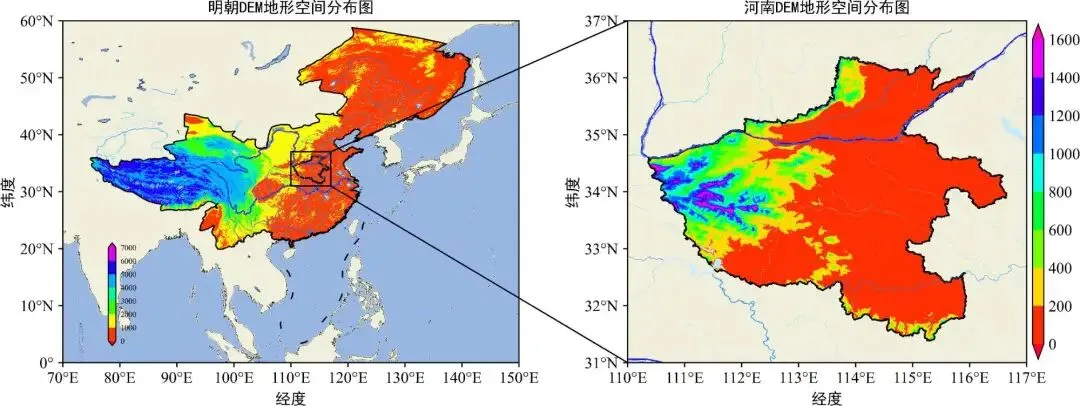
import numpy as npimport matplotlib.pyplot as pltimport cartopy.crs as ccrsimport cartopy.feature as cfeaturefrom cartopy.io.shapereader import Readerfrom cartopy.mpl.ticker import LongitudeFormatter,LatitudeFormatterimport xarray as xrimport rioxarray as rxrimport maskoutfrom matplotlib import rcParamsconfig = {"font.family":'Times New Roman',"font.size": 12,"mathtext.fontset":'stix'}rcParams.update(config)region=[70, 150, 0, 60]filename=r'./ETOPO2022.tif'ds = rxr.open_rasterio(filename)lons,lats = np.meshgrid(ds['x'],ds['y'])dem = ds[0]# plotfig=plt.figure(dpi=600,figsize=(16,9))proj=ccrs.PlateCarree()ax=fig.add_axes([0,0,0.4,0.4],projection=proj)ax.set_extent(region, crs = proj)ax.set_xticks(np.arange(region[0], region[1] + 1, 10), crs = proj)ax.set_yticks(np.arange(region[-2], region[-1] + 1, 10), crs = proj)ax.xaxis.set_major_formatter(LongitudeFormatter(zero_direction_label=False))ax.yaxis.set_major_formatter(LatitudeFormatter())ax.add_feature(cfeature.OCEAN.with_scale('50m'))ax.add_feature(cfeature.LAND.with_scale('50m'))ax.add_feature(cfeature.LAKES.with_scale('50m'))ax.add_geometries(Reader(r'./river1.shp').geometries(),ccrs.PlateCarree(),facecolor='none',edgecolor='b',linewidth=1)ax.add_geometries(Reader(r'./ming.shp').geometries(),ccrs.PlateCarree(),facecolor='none',edgecolor='k',linewidth=1)ax.add_geometries(Reader(r'./henan_province.shp').geometries(),ccrs.PlateCarree(),facecolor='none',edgecolor='k',linewidth=1)ax.add_geometries(Reader(r'./nineline.shp').geometries(),ccrs.PlateCarree(),facecolor='none',edgecolor='k',linewidth=1)ax.add_geometries(Reader(r'./ne_10m_land.shp').geometries(),ccrs.PlateCarree(),facecolor='none',edgecolor='k',linewidth=0.2)ax.add_geometries(Reader(r'./ne_50m_lakes.shp').geometries(),ccrs.PlateCarree(),facecolor='none',edgecolor='k',linewidth=0.2)ax.add_geometries(Reader(r'./henan1.shp').geometries(),ccrs.PlateCarree(),facecolor='none',edgecolor='k',linewidth=1.2,zorder=1)ax.add_geometries(Reader(r'./river1.shp').geometries(),ccrs.PlateCarree(),facecolor='none',edgecolor='b',linewidth=0.2)ax.add_geometries(Reader(r'./ne_50m_lakes.shp').geometries(),ccrs.PlateCarree(),facecolor='none',edgecolor='k',linewidth=0.2)ax.add_geometries(Reader(r'./1级河流.shp').geometries(),ccrs.PlateCarree(),facecolor='none',edgecolor='RoyalBlue',linewidth=0.4)ax.add_geometries(Reader(r'./2级河流.shp').geometries(),ccrs.PlateCarree(),facecolor='none',edgecolor='DodgerBlue',linewidth=0.3)ax.add_geometries(Reader(r'./3级河流.shp').geometries(),ccrs.PlateCarree(),facecolor='none',edgecolor='DeepSkyBlue',linewidth=0.2)ax.add_geometries(Reader(r'./4级河流.shp').geometries(),ccrs.PlateCarree(),facecolor='none',edgecolor='SkyBlue',linewidth=0.15)ax.add_geometries(Reader(r'./5级河流.shp').geometries(),ccrs.PlateCarree(),facecolor='none',edgecolor='LightSkyBlue',linewidth=0.05)ax.add_geometries(Reader(r'./主要湖泊.shp').geometries(),ccrs.PlateCarree(),edgecolor='none',linewidth=0,facecolor='#BEE8FF')c11=ax.contourf(lons,lats,dem,np.arange(0,8000,1000),extend='both',transform=ccrs.PlateCarree(),cmap='gist_rainbow',zorder=0)maskout(c11,ax,'./ming.shp',1)font3={'family':'SimHei','size':12,'color':'k'}plt.ylabel("纬度",fontdict=font3)plt.xlabel("经度",fontdict=font3)position=fig.add_axes([0.08,0.02,0.005,0.12])#位置[左,下,右,上]cbar=plt.colorbar(c11,cax=position,shrink=0.4,aspect=100,fraction=.03,pad=0.01)   #aspect控制bar宽度，fraction控制大小比例,pad控制与图的距离cbar.set_ticks(np.arange(0,8000,1000))        #设置colorbar范围和刻度标记间隔cbar.ax.tick_params(labelsize=6,direction='in',right=False)font3={'family':'SimHei','size':12,'color':'k'}ax.set_title('明朝DEM地形空间分布图',fontdict=font3)ax2=fig.add_axes([0.3,0,0.4,0.4],projection=proj)region2=[110,117,31,37]ax2.set_extent(region2, crs = proj)# ax.coastlines(scale, linewidth = 0.5)ax2.set_xticks(np.arange(region2[0], region2[1] + 1, 1), crs = proj)ax2.set_yticks(np.arange(region2[-2], region2[-1] + 1, 1), crs = proj)ax2.xaxis.set_major_formatter(LongitudeFormatter(zero_direction_label=False))ax2.yaxis.set_major_formatter(LatitudeFormatter())ax2.add_feature(cfeature.OCEAN.with_scale('50m'))ax2.add_feature(cfeature.LAND.with_scale('50m'))ax2.add_feature(cfeature.LAKES.with_scale('50m'))ax2.add_geometries(Reader(r'./river1.shp').geometries(),ccrs.PlateCarree(),facecolor='none',edgecolor='b',linewidth=1)ax2.add_geometries(Reader(r'./ming.shp').geometries(),ccrs.PlateCarree(),facecolor='none',edgecolor='k',linewidth=1)ax2.add_geometries(Reader(r'./henan_province.shp').geometries(),ccrs.PlateCarree(),facecolor='none',edgecolor='k',linewidth=1)ax2.add_geometries(Reader(r'./nineline.shp').geometries(),ccrs.PlateCarree(),facecolor='none',edgecolor='k',linewidth=1)ax2.add_geometries(Reader(r'./ne_10m_land.shp').geometries(),ccrs.PlateCarree(),facecolor='none',edgecolor='k',linewidth=0.2)ax2.add_geometries(Reader(r'./ne_50m_lakes.shp').geometries(),ccrs.PlateCarree(),facecolor='none',edgecolor='k',linewidth=0.2)ax2.add_geometries(Reader(r'./henan1.shp').geometries(),ccrs.PlateCarree(),facecolor='none',edgecolor='k',linewidth=1.2,zorder=1)ax2.add_geometries(Reader(r'./river1.shp').geometries(),ccrs.PlateCarree(),facecolor='none',edgecolor='b',linewidth=0.2)ax2.add_geometries(Reader(r'./ne_50m_lakes.shp').geometries(),ccrs.PlateCarree(),facecolor='none',edgecolor='k',linewidth=0.2)ax2.add_geometries(Reader(r'./1级河流.shp').geometries(),ccrs.PlateCarree(),facecolor='none',edgecolor='RoyalBlue',linewidth=0.4)ax2.add_geometries(Reader(r'./2级河流.shp').geometries(),ccrs.PlateCarree(),facecolor='none',edgecolor='DodgerBlue',linewidth=0.3)ax2.add_geometries(Reader(r'./3级河流.shp').geometries(),ccrs.PlateCarree(),facecolor='none',edgecolor='DeepSkyBlue',linewidth=0.2)ax2.add_geometries(Reader(r'./4级河流.shp').geometries(),ccrs.PlateCarree(),facecolor='none',edgecolor='SkyBlue',linewidth=0.15)ax2.add_geometries(Reader(r'./5级河流.shp').geometries(),ccrs.PlateCarree(),facecolor='none',edgecolor='LightSkyBlue',linewidth=0.05)ax2.add_geometries(Reader(r'./主要湖泊.shp').geometries(),ccrs.PlateCarree(),edgecolor='none',linewidth=0,facecolor='#BEE8FF')c12=ax2.contourf(lons,lats,dem,np.arange(0,1800,200),extend='both',transform=ccrs.PlateCarree(),cmap='gist_rainbow',zorder=0)maskout(c12,ax2,'./henan_province.shp',1)cbar=plt.colorbar(c12,shrink=0.98,aspect=30,fraction=.03,pad=0.01)   #aspect控制bar宽度，fraction控制大小比例,pad控制与图的距离cbar.set_ticks(np.arange(0,1800,200))         #设置colorbar范围和刻度标记间隔cbar.ax.tick_params(labelsize=12, direction='in', right=False)font3={'family':'SimHei','size':12,'color':'k'}ax2.set_title('河南DEM地形空间分布图',fontdict=font3)font3={'family':'SimHei','size':12,'color':'k'}plt.ylabel("纬度",fontdict=font3)plt.xlabel("经度",fontdict=font3)ax.plot([110,117,117,110,110],[31,31,37,37,31],lw=1,transform=ccrs.PlateCarree(),color='k')import matplotlib.patches as mpatchestrans_proj=ccrs.PlateCarree()#用于转换的原坐标target_proj=ccrs.PlateCarree()x=np.array([117,117])y=np.array([37,31])x2=np.array([110,110])for m,n,h,j in zip(x,y,x2,y):#由于移动了中心坐标轴，此处的x转化需减去这个值    xyA=target_proj.transform_point(m,n,trans_proj)    xyB=[h,j]    con=mpatches.ConnectionPatch(    xyA=xyA,xyB=xyB,coordsA=ax.transData,coordsB=ax2.transData,color='k',ls='-')    fig.add_artist(con)plt.savefig('./plot280.1.png',dpi=800,bbox_inches='tight',pad_inches=0)plt.show()

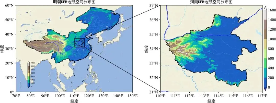
c11=ax.contourf(lons,lats,dem,np.arange(0,8000,1000),extend='both',transform=ccrs.PlateCarree(),cmap=cmaps.MPL_terrain,zorder=0)

给大家送本书：

《MATLAB×AI：科研绘图与学术图表智能绘制一本通》

编辑推荐：

本书旨在介绍如何借助DeepSeek更高效地进行MATLAB学术图表的绘制。全书首先介绍MATLAB与DeepSeek的基础知识，以及学术图表的基本规范；接着详细介绍MATLAB学术图表的绘制流程与图形元素组成；最后系统讲解折线图、柱状图、散点图、三维曲面图及特殊绘图等常见学术图表的绘制方法。书中共包含21个DeepSeek应用案例，它们作为相关章节内容的补充与延伸，同时用于展示AI在绘图过程中的多样化应用思路。

本书适合MATLAB与DeepSeek零基础的在校学生、科研人员，以及对数据可视化感兴趣的各领域读者学习使用。此外，本书也适用于具备一定编程基础，但在图表审美与规范方面有所欠缺，并希望系统提升绘图能力的读者。

抽奖方式及满足条件：

1.关注气象水文科研猫；

2.转发本文到朋友圈；

3.给本文点【赞】、点【在看】；

4.留言区评论点赞最多者。

同时满足上述4个条件的留言区点赞前4名的读者，

每人免费包邮一本：

《MATLAB×AI：科研绘图与学术图表智能绘制一本通》。

开奖日期：2026年5月25日晚8点。