Python绘图 | NC小提琴图复现(包含完整代码)
- 2026-10-11 06:07:26
Python绘图 | NC小提琴图复现(包含完整代码)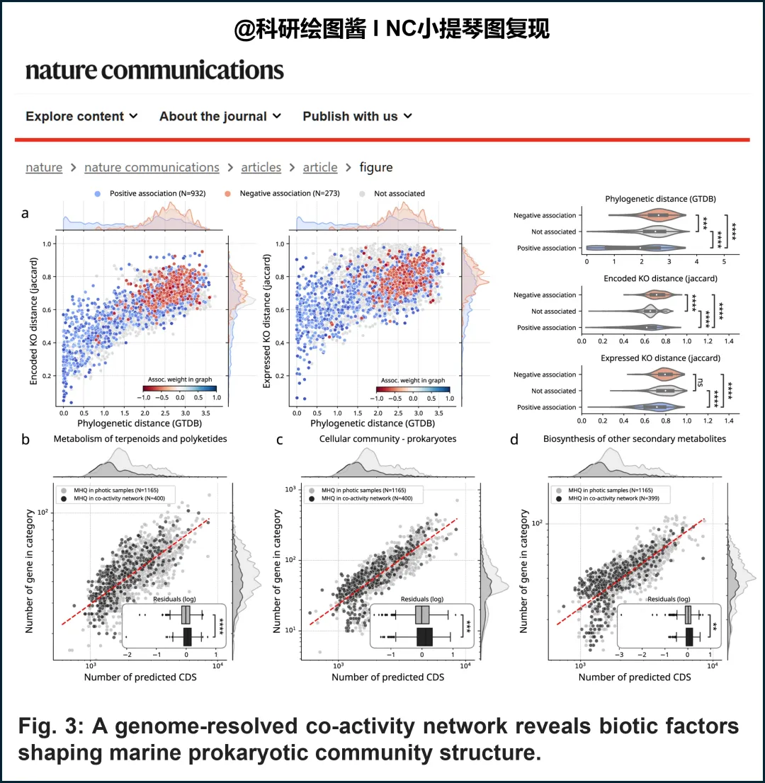
复现前后对比: 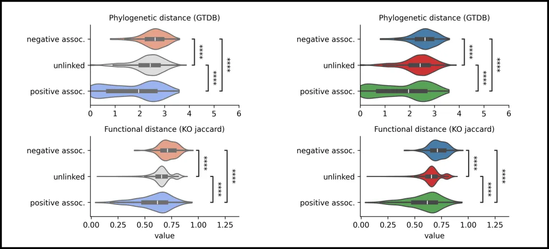
下面展示了如何用Python复现的过程(数据来源于文章的源数据)。 1. 加载绘图相关的依赖包: 2. 设置绘图参数: 3. 绘图函数设置: 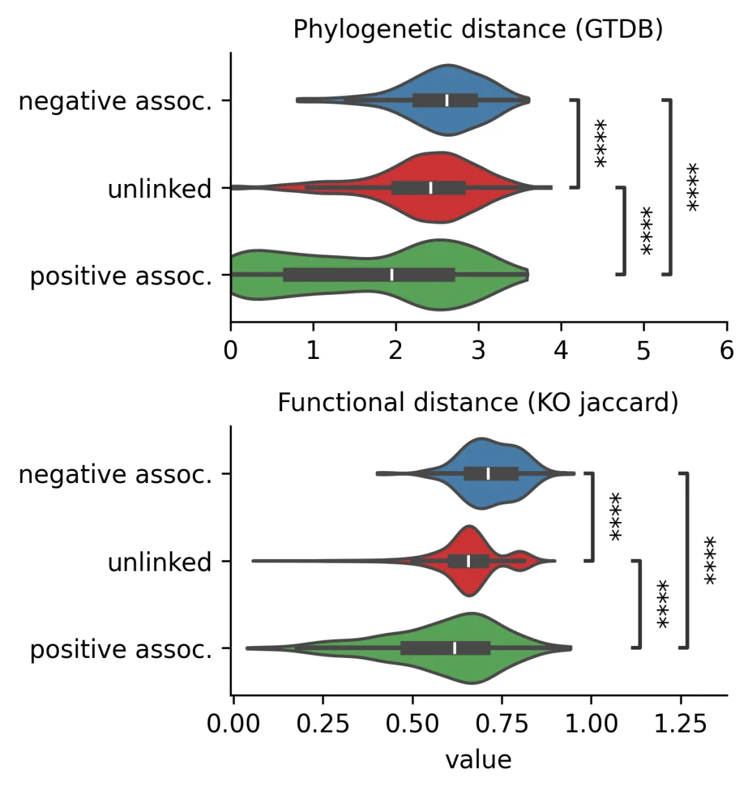
好了,本期内容到此结束,喜欢的小伙伴可以转发分享,收藏,别忘了来个三连击啊~~~ Python绘图 | 复现顶刊中机器学习SHAP特征重要性交互网络与个性化解释图(包含完整代码) R绘图 | Science网络相关性热图复现(包含完整代码) R绘图 | NC相关性矩阵热图复现(包含完整代码) R绘图 | CNS 级相关性矩阵热图复现进阶教程(含完整代码) Python绘图 | Nature不同细胞类型中标记基因的表达点图复现(包含完整代码) R绘图 | Nature山脊图复现(包含完整代码) R绘图 | Nature散点配对连线图(包含完整代码) Python绘图 | NC变量相关性散点图复现(包含完整代码) R绘图 | NC主成分PCA图复现(包含完整代码)

添加小编微信进群交流学习!
小提琴图可同时展示数据分布的概率密度形状与关键分位数,适用于探测多模态、偏态等复杂分布特征,多用于探索性数据分析。箱线图则专注于呈现中位数、四分位距及异常值,侧重于统计摘要的稳健比较,适用于样本量较小或需简洁展示多组差异的场景。二者核心差异在于信息维度:箱线图仅反映分布位置与尺度,而小提琴图额外揭示分布形态。实践中建议先以小提琴图识别数据潜在结构,再辅以箱线图进行组间统计量对比。原图源于Nature Communications杂志上的一篇文献:Genome-scale community modelling reveals conserved metabolic cross-feedings in epipelagic bacterioplankton communities。下面展示了Python绘制这类图的全部过程,供大家参考。
原文中的结果图:Fig. 3
Python代码
import pandas as pdimport ete3import scipy as sciimport numpy as npimport osimport seaborn as snsimport matplotlib as mplimport matplotlib.pyplot as pltimport mpl_toolkits.axes_grid1.inset_locatorfrom statannotations.Annotator import Annotatorimport itertoolsimport randomrandom.seed(0)
funvsphyl_dir = "./Fig/"%matplotlib inlinempl.rcParams['figure.dpi'] = 300mpl.rcParams['savefig.dpi'] = 300plt.rcParams['svg.fonttype'] = "none"CELL_COLORS = {"negative assoc.": "#377EB8", # 蓝色"unlinked": "#E41A1C", # 红色"positive assoc.": "#4DAF4A", # 绿色}
palette_colors = [CELL_COLORS[cat] for cat in order]df = pd.read_csv('./dataset.csv')new_categories = ("unlinked","positive assoc.","negative assoc.",)order = (new_categories[2], new_categories[0], new_categories[1])g_r = sns.catplot(data=df.set_index(["genome_a", "genome_b", "category"]).drop(columns="edge").melt(ignore_index=False).reset_index(),kind="violin",row="variable",x="value",y="category",palette=palette_colors, # 使用CELL经典颜色order=order,height=4.5 / 2,aspect=2,sharex=False,cut=0,)# 定义 graphtype 变量graphtype = "dRep95_MHQ"# Add annotations for significance for Mann-Whitney U testpairs = list(itertools.combinations(order, 2))for i, ax in enumerate(g_r.axes.flatten()):ax.set_title(ax.get_title().split("= ", 1)[1], fontsize=10)ax.set_ylabel(None)print(ax.get_title())boxplot_args = dict(data=df,x=ax.get_title(),y="category",palette=palette_colors, # 使用CELL经典颜色order=order,)annotator = Annotator(ax=ax,pairs=pairs,**boxplot_args,orient="h",)annotator.configure(test="Mann-Whitney",text_format="star",loc="inside",verbose=1,comparisons_correction="Bonferroni",)_, _ = annotator.apply_and_annotate()if i == 0:ax.set_xlim(0, 6)# 保存图片for ext in ("svg", "pdf", "png"):os.makedirs(os.path.join(funvsphyl_dir, ext), exist_ok=True)g_r.figure.savefig(os.path.join(funvsphyl_dir,ext,f"dRep95_MHQ_fundist-vs-phyldist-tests_{graphtype}.{ext}",),bbox_inches="tight",dpi=300,)plt.show()
复现图如下
往期回顾
参考文献:Giordano, N., Gaudin, M., Trottier, C. et al. Genome-scale community modelling reveals conserved metabolic cross-feedings in epipelagic bacterioplankton communities. Nat Commun 15, 2721 (2024). https://doi.org/10.1038/s41467-024-46374-w
以上内容为原创,转载需声明出处。
🔥亲测有效,一键运行,助你快速上手!
🔥整理不易,欢迎点赞分享给更多小伙伴~
本文来自网友投稿或网络内容,如有侵犯您的权益请联系我们删除,联系邮箱:596563534@qq.com 。
随机文章
-
 10个月宝宝每天需要喝多少奶粉?
- Pywin32:用Python高效快速访问Windows系统底层 API,简化你的Windows自动化任务
- NO.XC008全国初中信息技术说课《Python分支结构-社会实践篇》(说课课件+说课稿+教学设计+说课上课视频)2022七上
- Linux PM 日报 | 2026-05-27 · 23 patches
- Python os 模块完全指南:从 cwd 到系统操作,一文掌握文件与路径管理
- Linux 最新资讯 20260602——X.Org Server 六月曝出九项AI发现的新安全漏洞;COSMIC Desktop 的毛玻璃带来 Windows Aero 风格
- 花2个小时,从0到1;邪修速通Linux秘籍!
- 好消息是TodoList快捷键功能在Linux端调通了,坏消息调试过程在Mac端把python环境搞崩了[苦涩]关键目前完全不晓得咋崩的,陷入沉思中…
- 一图总结Python常用的第三方库
- 王炸!Kafka 4.0 重磅发布,Java 8 和 Zookeeper 彻底被抛弃了..一个时代结束了!
- Linux搭建MySQL主从集群