期刊图片复现|Python绘制多面板哑铃图
- 2026-10-11 06:01:49
期刊图片复现|Python绘制多面板哑铃图

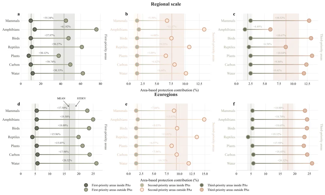
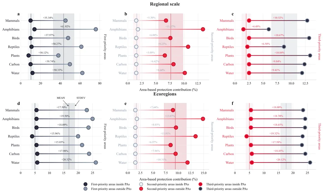
论文:Targeted Synergistic Priorities for Conserving Biodiversity,Carbon, and Water on the Qinghai‐Tibetan Plateau 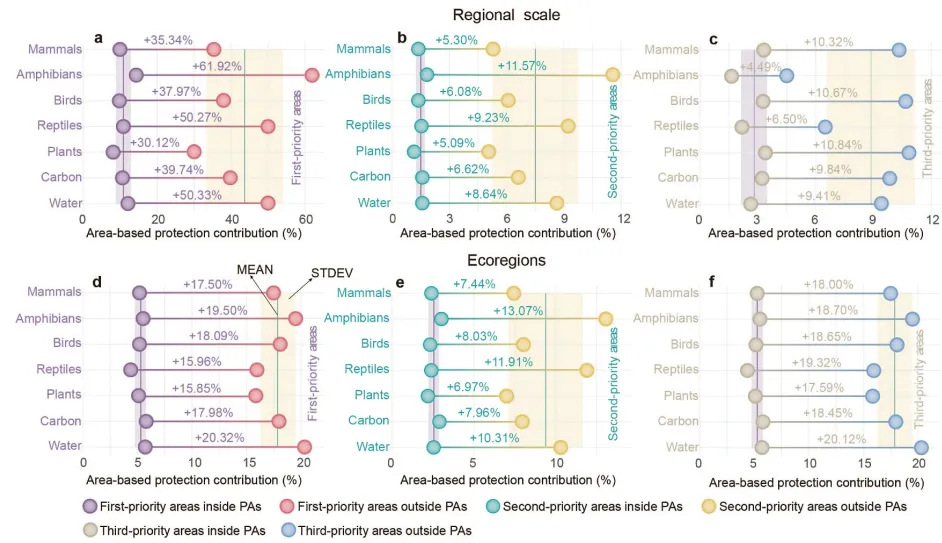
论文原图 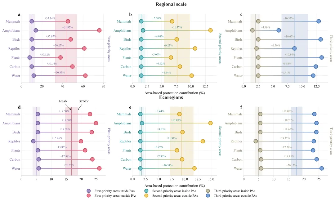
仿图 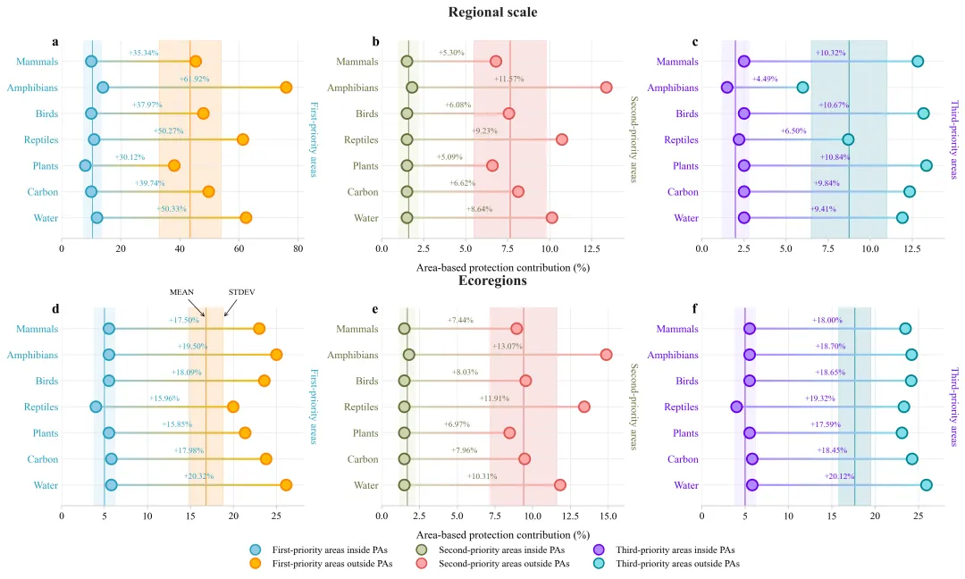
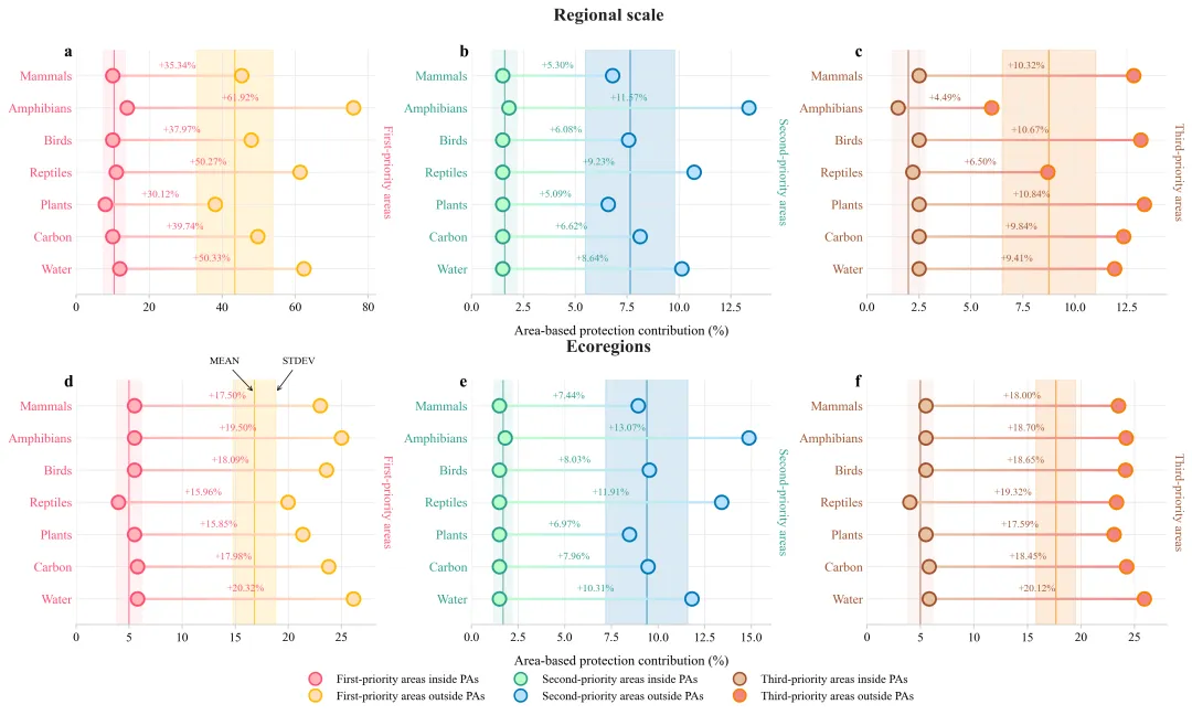
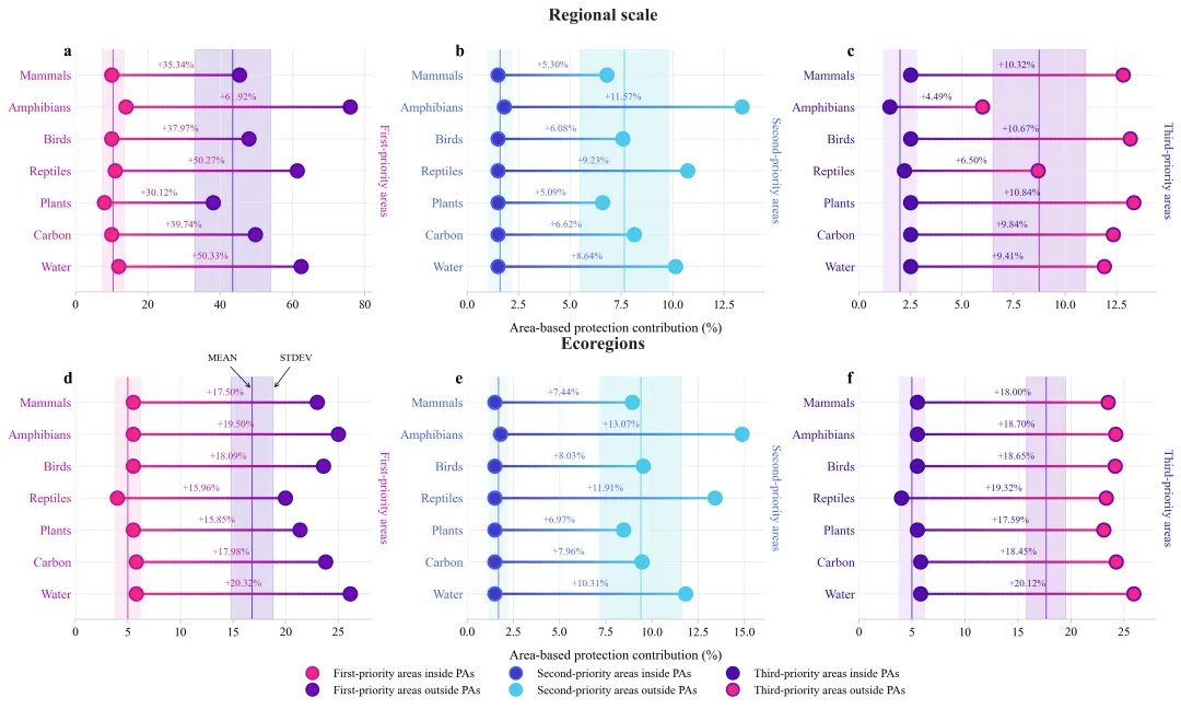
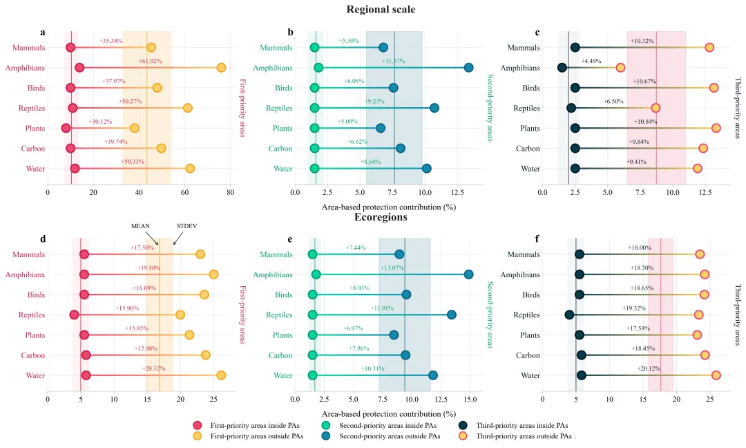
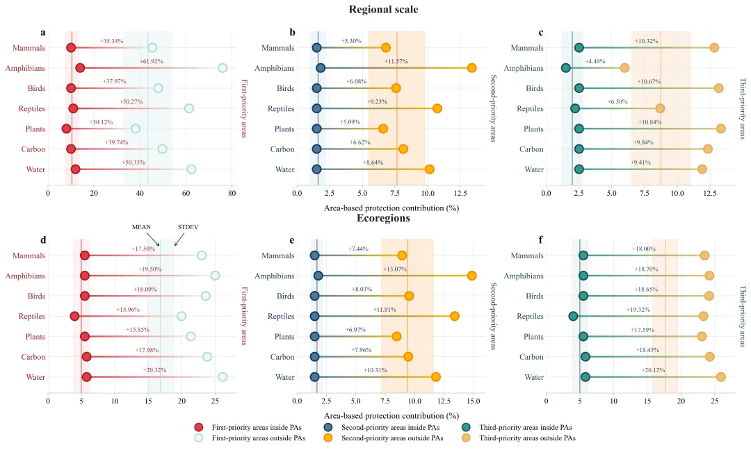
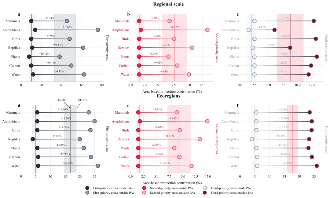
多种配色 



库的导入以及字体设置 

设置颜色库 

绘图函数:函数初始化与画布创建 

绘图函数:数据准备、颜色提取 

绘图函数:绘制标准差阴影区间、均值线、网格线 

绘图函数:绘制哑铃图 

绘图函数:刻度样式设置、均值、标准差标注添加 

绘图函数:标题设置、图例设置、布局调整、绘图结果保存 
执行部分:读取数据、设置是否进行批量绘图 



期刊图片复现|Python绘制二维偏依赖PDP图 期刊复现|python绘制基于SHAP分析和GAM模型拟合的单特征依赖图 期刊图片复现|python绘制带有渐变颜色shap特征重要性组合图(条形图+蜂巢图) 期刊复现|用Python绘制SHAP特征重要性总览图、依赖图、双特征交互效应SHAP图,解锁XGBoost模型的终极奥秘 期刊图片复现|Python绘制shap重要性蜂巢图+单特征依赖图+交互效应强度气泡图+交互效应依赖图(回归+二分类+分类) 

公众号中的所有所有的免费代码都已经下架了,都并入到付费部分里了,付费合集代码和数据的购买通道已经开通,全部合集100元,后续将会持续更新,决定购买请后台私信我,注意只会分享练习数据和代码文件,不会提供答疑服务,代码文件中已经包含了每行代码的完整注释,购买前请确保真的需要!!!
代码绘制成果展示
代码解释
第一部分
# =========================================================================================# ====================================== 1. 环境设置 =======================================# =========================================================================================import osimport numpy as npimport pandas as pdimport matplotlib.pyplot as plt
第二部分
# =========================================================================================# ======================================2.颜色库============================================# =========================================================================================COLOR_SCHEMES = {1: ['#a28ec4', '#725a9c', '#ea8093', '#c84860', '#f1ecf6', '#6ec2c7', '#2f878c', '#f3d067', '#ca9e27', '#eef7f8','#c6bfa7', '#8c8468', '#7ca3d9', '#416ea8', '#f5f4ef'],}
第三部分
# =========================================================================================# ======================================3.绘图函数============================================# =========================================================================================def plot_advanced_forest_chart(df, scheme_id):labels = df['Feature'].unique().tolist() #特征名称scales = df['Scale'].unique().tolist() #分组priorities = df['Priority'].unique().tolist() #阶段y_pos = np.arange(len(labels))[::-1] #生成y轴坐标cfg_scheme = COLOR_SCHEMES[scheme_id] #提取配色方案#创建画布fig, axs = plt.subplots(len(scales), len(priorities), figsize=(15.5, 9.0))
第四部分
# 遍历行for row_idx in range(len(scales)):# 遍历列for col_idx in range(len(priorities)):ax = axs[row_idx, col_idx] #获取当前子图current_scale = scales[row_idx] #组名current_priority = priorities[col_idx] #阶段名key_letter = chr(97 + row_idx * len(priorities) + col_idx) #子图编号ax.set_xlim(0, max(df_panel['Outside']) * 1.08) #x轴范围
第五部分
#左侧阴影ax.axvspan(mean_l - stdev_l, #xmean_l + stdev_l, #ycolor=b_l_color, #背景色alpha=0.9, #透明度zorder=0) #层#网格线ax.grid(True, # 开启which='both', #xycolor='#eaeaea', #颜色linestyle='-', #样式linewidth=0.8, #线宽zorder=1) #层ax.set_axisbelow(True) #设置在最底下
第六部分
#创建渐变色cmap_gradient = LinearSegmentedColormap.from_list('line_grad', [c_in_f, c_out_f])#右侧点ax.scatter(x2, #xy, #yfacecolor=c_out_f,#填充色edgecolor=c_out_e,#边缘色s=140, #散点大小linewidths=1.8, #边粗细zorder=3) #层#差值文本ax.text((x1 + x2) / 2, #xy + 0.16, #ydiff_txt, #文本ha='center', #水平va='bottom', #垂直color=c_in_e, #字体颜色fontsize=9, #大小fontweight='normal') #粗细
第七部分
ax.set_yticks(y_pos) #y轴刻度位置#配置y轴刻度ax.tick_params(axis='y', #ywhich='both', #主副刻度length=0, #长labelsize=11.5, #字体大小labelcolor=c_in_e) #字体颜色ax.set_yticklabels(labels) #添加y轴特征名if key_letter == 'd':ax.annotate('MEAN', #文本xy=(16.8, 6.4), #箭头终点xytext=(14.0, 7.3), #文本位置arrowprops=dict(arrowstyle="->", #箭头color="black", #黑色lw=0.7), #线宽fontsize=9, #字体大小ha='center') #水平ax.annotate('STDEV', #文本xy=(18.8, 6.4), #箭头终点xytext=(21.0, 7.3), #文本位置arrowprops=dict(arrowstyle="->", #箭头color="black", #黑色lw=0.7), #线宽fontsize=9, #字体大小ha='center') #水平
第八部分
#设置组标题fig.text(0.5, #x0.95, #yscales[0], #文本ha='center', #水平fontsize=16, #大小fontweight='bold', #加粗color='#222222') #颜色fig.text(0.5, #x0.50, #yscales[1], #文本ha='center', #水平fontsize=16, #大小fontweight='bold',#加粗color='#222222') #颜色#添加图例fig.legend(handles=legend_elements, #句柄loc='lower center', #位置ncol=3, #列frameon=False, #去掉边框fontsize=10.5, #字体大小bbox_to_anchor=(0.5, 0.01)) #坐标
第九部分
# =========================================================================================# ======================================4.执行部分============================================# =========================================================================================if __name__ == '__main__':data_path = r'data.xlsx' #原始数据df_real = pd.read_excel(data_path) #读取数据else:scheme_id = 1print('正在绘制并保存方案:', scheme_id)plot_advanced_forest_chart(df_real, scheme_id)
如何应用到你自己的数据
1.设置原始数据的保存路径,执行部分:
data_path = r'data.xlsx' #原始数据2.设置是否进行批量绘图,执行部分:
plot_all = True #是否批量绘图3.设置绘图结果保存地址,绘图函数部分:
plt.savefig(fr'{scheme_id}.pdf',bbox_inches='tight')推荐
获取方式
本文来自网友投稿或网络内容,如有侵犯您的权益请联系我们删除,联系邮箱:596563534@qq.com 。
随机文章
-
 10个月宝宝每天需要喝多少奶粉?
- Python 数据分析基础入门:《Excel Python:飞速搞定数据分析与处理》学习笔记系列(附录 C 高级 概念)
- 一张图汇总Linux安全工具合集!
- Arch Linux安装Claude Code记录
- AI大模型底层逻辑揭秘:深度解析Python、C++等编程语言如何驱动智能革命
- Python 3.14 软件官方安装包及安装教程(附全部版本安装包)
- 暑假班|计算机二级+Python通关班,带你轻松拿证!
- Python对同一文件夹多工作簿进行合并
- Python 纯算还原快手签名,17 个接口实测通过,关键过程复盘
- 有关于Python的一些认知!
- 职场提效神器:16组万能Python自动化代码