【生信分析】Python-2.序列比对-基于Smith-Waterman动态规划算法的局部比对
- 2026-06-28 05:54:49

生物信息学分析(生信分析)是结合生物学、计算机科学和统计学,对生物数据进行处理、挖掘和解释的多学科领域。其核心思想是通过计算手段从海量数据(如基因组、转录组、蛋白质组数据)中提取生物学洞见,从而解决疾病机制、基因功能、进化关系等问题。


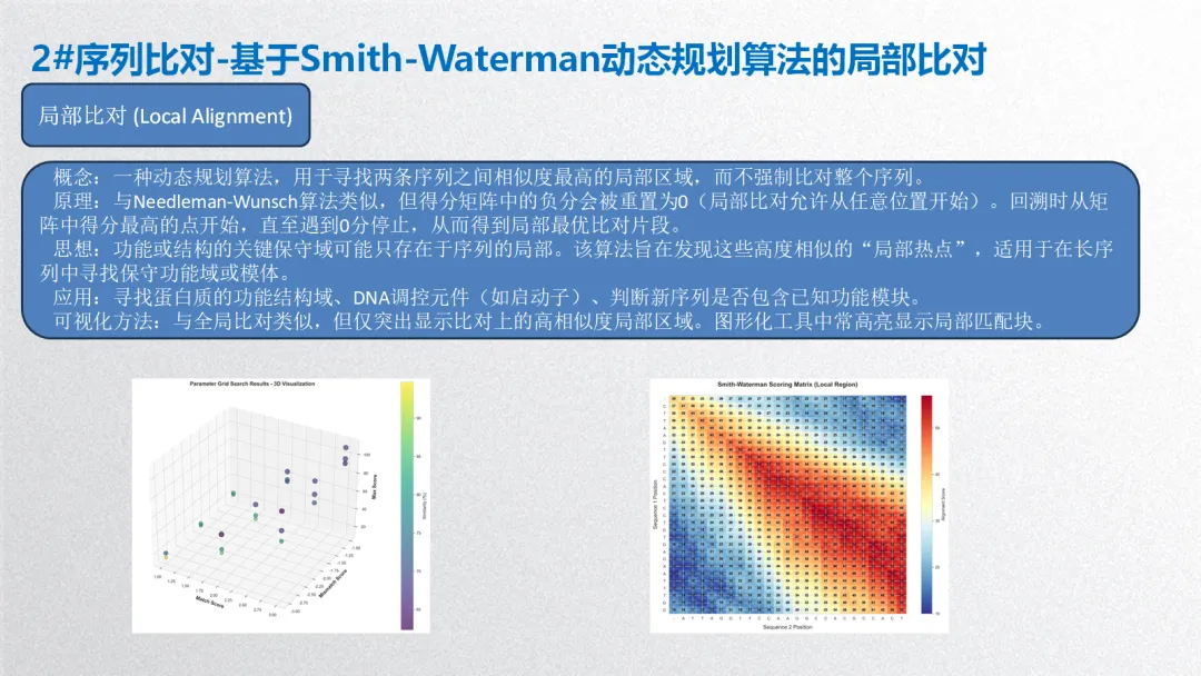
2. 序列比对-基于Smith-Waterman动态规划算法的局部比对
概念:一种动态规划算法,用于寻找两条序列之间相似度最高的局部区域,而不强制比对整个序列。
原理:与Needleman-Wunsch算法类似,但得分矩阵中的负分会被重置为0(局部比对允许从任意位置开始)。回溯时从矩阵中得分最高的点开始,直至遇到0分停止,从而得到局部最优比对片段。
思想:功能或结构的关键保守域可能只存在于序列的局部。该算法旨在发现这些高度相似的“局部热点”,适用于在长序列中寻找保守功能域或模体。
应用:寻找蛋白质的功能结构域、DNA调控元件(如启动子)、判断新序列是否包含已知功能模块。
可视化方法:与全局比对类似,但仅突出显示比对上的高相似度局部区域。图形化工具中常高亮显示局部匹配块。
生信分析可按照分析目的和数据层次分为以下几个主要方面:
1. 序列分析
2. 结构分析
3. 比较基因组学与进化分析
4. 转录组学与基因表达分析
5. 表观基因组学
6. 蛋白质组学与互作网络
7. 单细胞组学
8. 整合多组学与系统生物学
9. 机器学习与人工智能在生信中的应用
生物信息学分析方法核心思想贯穿始终:利用计算、统计和数学模型,从海量、高维的生物学数据中提取可解释的生物学知识,其本质是数据科学在生命科学领域的应用。以下基于常见研究流程,将生信分析方法分为 5 个主要方面,并详细介绍各类方法的概念、原理、思想、应用及可视化方式。
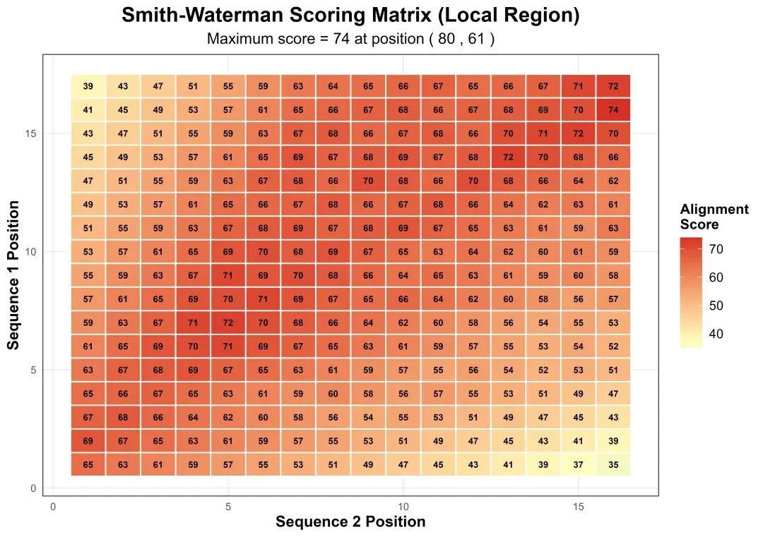
# pip install numpy pandas matplotlib seaborn scikit-learn openpyxl Pillow# ============================================================================# 生物信息学分析:Smith-Waterman局部比对完整分析流程(Python实现)# 描述:Python实现SW局部比对,包含完整的数据分析、模型构建与评价、可视化及报告生成# ============================================================================import osimport randomimport numpy as npimport pandas as pdimport matplotlib.pyplot as pltimport seaborn as snsfrom matplotlib.gridspec import GridSpecfrom datetime import datetimeimport warningswarnings.filterwarnings('ignore')# 设置中文字体支持plt.rcParams['font.sans-serif'] = ['SimHei', 'DejaVu Sans']plt.rcParams['axes.unicode_minus'] = False# -------------------- 第一部分:环境初始化 --------------------print("步骤1:初始化环境...")# 设置随机种子保证结果可重复random.seed(20250104)np.random.seed(20250104)# 创建结果目录desktop_path = os.path.expanduser("~/Desktop")results_dir = os.path.join(desktop_path, "02_LA_Results")if not os.path.exists(results_dir): os.makedirs(results_dir)print(f"创建结果目录: {results_dir}")else:print(f"结果目录已存在: {results_dir}")print(f"工作目录: {desktop_path}")print(f"结果将保存至: {results_dir}\n")# -------------------- 第二部分:模拟序列数据生成 --------------------print("步骤2:生成模拟DNA序列数据...")# 定义核苷酸字符集nucleotides = ["A", "T", "C", "G"]# 生成两条长度不同的模拟DNA序列(局部比对需要不同长度)seq1_length = 80 # 第一条序列长度seq2_length = 60 # 第二条序列长度# 序列1:随机生成sequence_1 = "".join(random.choices(nucleotides, k=seq1_length))# 序列2:生成包含序列1局部区域的序列# 在序列1中随机选取一段作为保守区域conserved_start = random.randint(10, 40)conserved_length = 30conserved_region = sequence_1[conserved_start:conserved_start + conserved_length]# 在保守区域周围添加随机序列left_flank = "".join(random.choices(nucleotides, k=15))right_flank = "".join(random.choices(nucleotides, k=15))# 在保守区域引入一些突变def mutate_conserved(seq, mutation_rate=0.15): seq_list = list(seq)for i in range(len(seq_list)):if random.random() < mutation_rate: possible_sub = [n for n in nucleotides if n != seq_list[i]]if possible_sub: seq_list[i] = random.choice(possible_sub)return"".join(seq_list)conserved_mutated = mutate_conserved(conserved_region)sequence_2 = left_flank + conserved_mutated + right_flank# 确保序列2长度正确if len(sequence_2) > seq2_length: sequence_2 = sequence_2[:seq2_length]elif len(sequence_2) < seq2_length: extra = "".join(random.choices(nucleotides, k=seq2_length - len(sequence_2))) sequence_2 = sequence_2 + extraprint("模拟序列生成完成。")print(f"序列1 (长度={len(sequence_1)}): {sequence_1[:40]}...")print(f"序列2 (长度={len(sequence_2)}): {sequence_2[:40]}...")print(f"保守区域在序列1中的位置: {conserved_start}-{conserved_start + conserved_length - 1}\n")# 将序列保存为FASTA格式fasta_content = f""">Sequence_1_Simulated_Local_Alignment{sequence_1}>Sequence_2_Simulated_Local_Alignment{sequence_2}"""fasta_path = os.path.join(results_dir, "simulated_sequences_local.fasta")with open(fasta_path, "w") as f: f.write(fasta_content)print(f"FASTA序列已保存: {fasta_path}\n")# -------------------- 第三部分:Smith-Waterman算法实现 --------------------print("步骤3:执行Smith-Waterman局部比对...")# 定义比对参数match_score = 2mismatch_score = -1gap_penalty = -2def smith_waterman(seq1, seq2, match_score, mismatch_score, gap_penalty):"""Smith-Waterman局部比对算法实现""" seq1_chars = list(seq1) seq2_chars = list(seq2) n = len(seq1) + 1 # 行数 m = len(seq2) + 1 # 列数# 初始化得分矩阵和回溯矩阵 score_matrix = np.zeros((n, m), dtype=int) trace_matrix = np.zeros((n, m), dtype=int)# 回溯方向: 0=停止, 1=对角线, 2=向上, 3=向左 max_score = 0 max_i, max_j = 0, 0# 填充得分矩阵for i in range(1, n):for j in range(1, m):# 计算对角线得分(匹配或错配) char1 = seq1_chars[i - 1] char2 = seq2_chars[j - 1] diagonal_score = score_matrix[i - 1, j - 1] + (match_score if char1 == char2 else mismatch_score)# 计算上方得分(序列1空位) up_score = score_matrix[i - 1, j] + gap_penalty# 计算左方得分(序列2空位) left_score = score_matrix[i, j - 1] + gap_penalty# Smith-Waterman关键:取最大值,但不得小于0 scores = [0, diagonal_score, up_score, left_score] max_cell_score = max(scores) score_matrix[i, j] = max_cell_score trace_matrix[i, j] = scores.index(max_cell_score) # 记录方向索引# 记录最大得分和位置if max_cell_score > max_score: max_score = max_cell_score max_i, max_j = i, j# 回溯构建比对结果(从最大得分点开始) aligned_seq1 = [] aligned_seq2 = [] match_symbol = [] i, j = max_i, max_jwhile i > 0 and j > 0 and score_matrix[i, j] > 0: direction = trace_matrix[i, j]if direction == 1: # 对角线 aligned_seq1.insert(0, seq1_chars[i - 1]) aligned_seq2.insert(0, seq2_chars[j - 1]) match_symbol.insert(0, "|"if seq1_chars[i - 1] == seq2_chars[j - 1] else".") i -= 1 j -= 1elif direction == 2: # 向上 aligned_seq1.insert(0, seq1_chars[i - 1]) aligned_seq2.insert(0, "-") match_symbol.insert(0, " ") i -= 1elif direction == 3: # 向左 aligned_seq1.insert(0, "-") aligned_seq2.insert(0, seq2_chars[j - 1]) match_symbol.insert(0, " ") j -= 1else:break# 遇到0分停止# 整理比对结果if aligned_seq1: aligned_seq1_str = "".join(aligned_seq1) aligned_seq2_str = "".join(aligned_seq2) match_symbol_str = "".join(match_symbol)# 计算比对统计信息 total_length = len(aligned_seq1) matches = sum(1 for a, b in zip(aligned_seq1, aligned_seq2) if a == b and a != "-") mismatches = sum(1 for a, b in zip(aligned_seq1, aligned_seq2) if a != b and a != "-" and b != "-") gaps = sum(1 for a, b in zip(aligned_seq1, aligned_seq2) if a == "-" or b == "-") similarity = matches / total_length * 100 if total_length > 0 else 0# 计算局部比对的位置信息 seq1_start = i seq1_end = max_i - 1 seq2_start = j seq2_end = max_j - 1else: aligned_seq1_str = "" aligned_seq2_str = "" match_symbol_str = "" total_length = 0 matches = 0 mismatches = 0 gaps = 0 similarity = 0 seq1_start = 0 seq1_end = 0 seq2_start = 0 seq2_end = 0return {"seq1_aligned": aligned_seq1_str,"seq2_aligned": aligned_seq2_str,"match_symbol": match_symbol_str,"score_matrix": score_matrix,"trace_matrix": trace_matrix,"max_score": max_score,"max_position": (max_i, max_j),"alignment_range": {"seq1_start": seq1_start,"seq1_end": seq1_end,"seq2_start": seq2_start,"seq2_end": seq2_end },"statistics": {"total_length": total_length,"matches": matches,"mismatches": mismatches,"gaps": gaps,"similarity": similarity } }# 执行比对sw_result = smith_waterman(sequence_1, sequence_2, match_score, mismatch_score, gap_penalty)print("Smith-Waterman局部比对完成。")print(f"最大比对得分:{sw_result['max_score']}")print(f"比对长度:{sw_result['statistics']['total_length']}")print(f"匹配数:{sw_result['statistics']['matches']} ({sw_result['statistics']['similarity']:.2f}%)")print(f"错配数:{sw_result['statistics']['mismatches']}")print(f"空位数:{sw_result['statistics']['gaps']}")print(f"序列1比对区域:{sw_result['alignment_range']['seq1_start']}-{sw_result['alignment_range']['seq1_end']}")print(f"序列2比对区域:{sw_result['alignment_range']['seq2_start']}-{sw_result['alignment_range']['seq2_end']}\n")# -------------------- 第四部分:数据分析与模型构建 --------------------print("步骤4:进行数据分析与模型构建...")# 1. 生成比对质量评估数据# 创建不同参数下的比对结果比较param_grid = []match_scores = [1, 2, 3]mismatch_scores = [-1, -2, -3]gap_penalties = [-1, -2, -3]for match in match_scores:for mismatch in mismatch_scores:for gap in gap_penalties: param_grid.append({"match_score": match,"mismatch_score": mismatch,"gap_penalty": gap })alignment_results = []for i, params in enumerate(param_grid): result = smith_waterman(sequence_1, sequence_2, params["match_score"], params["mismatch_score"], params["gap_penalty"]) alignment_results.append({"Param_Set": i + 1,"Match_Score": params["match_score"],"Mismatch_Score": params["mismatch_score"],"Gap_Penalty": params["gap_penalty"],"Max_Score": result["max_score"],"Alignment_Length": result["statistics"]["total_length"],"Matches": result["statistics"]["matches"],"Similarity": result["statistics"]["similarity"],"Seq1_Start": result["alignment_range"]["seq1_start"],"Seq1_End": result["alignment_range"]["seq1_end"] })alignment_df = pd.DataFrame(alignment_results)# 2. 构建机器学习模型预测比对质量# 准备训练数据np.random.seed(20250104)# 使用相似度中位数作为阈值similarity_threshold = alignment_df["Similarity"].median()print(f"使用相似度中位数作为阈值:{similarity_threshold:.2f}")train_data = alignment_df.copy()train_data["High_Quality"] = (train_data["Similarity"] > similarity_threshold).astype(int)train_data = train_data.drop(["Param_Set", "Seq1_Start", "Seq1_End"], axis=1)# 检查类别分布high_quality_count = train_data["High_Quality"].sum()low_quality_count = len(train_data) - high_quality_countprint(f"高质量比对样本数:{high_quality_count}")print(f"低质量比对样本数:{low_quality_count}")# 尝试构建机器学习模型if high_quality_count >= 2 and low_quality_count >= 2: try: from sklearn.model_selection import train_test_split from sklearn.ensemble import RandomForestClassifier from sklearn.metrics import confusion_matrix, classification_report, accuracy_score from sklearn.linear_model import LassoCV from sklearn.preprocessing import StandardScaler# 准备特征和目标变量 X = train_data.drop("High_Quality", axis=1) y = train_data["High_Quality"]# 划分训练集和测试集 X_train, X_test, y_train, y_test = train_test_split(X, y, test_size=0.3, random_state=42)# 构建随机森林模型print("构建随机森林模型...") rf_model = RandomForestClassifier(n_estimators=200, random_state=42) rf_model.fit(X_train, y_train)# 模型预测 y_pred = rf_model.predict(X_test) y_pred_proba = rf_model.predict_proba(X_test)[:, 1]# 模型评估 rf_confusion = confusion_matrix(y_test, y_pred) rf_accuracy = accuracy_score(y_test, y_pred)# 计算敏感性、特异性 tn, fp, fn, tp = rf_confusion.ravel() rf_sensitivity = tp / (tp + fn) if (tp + fn) > 0 else 0 rf_specificity = tn / (tn + fp) if (tn + fp) > 0 else 0print("随机森林模型评估:")print(f"准确率:{rf_accuracy * 100:.2f}%")print(f"敏感性:{rf_sensitivity * 100:.2f}%")print(f"特异性:{rf_specificity * 100:.2f}%")# 构建LASSO回归模型选择重要特征print("构建LASSO回归模型...")# 标准化特征 scaler = StandardScaler() X_scaled = scaler.fit_transform(X)# 使用LASSO回归 lasso_model = LassoCV(cv=5, random_state=42, max_iter=10000) lasso_model.fit(X_scaled, y)# 提取重要特征 important_features = X.columns[lasso_model.coef_ != 0].tolist()if not important_features: important_features = ["Match_Score", "Mismatch_Score"] # 默认特征print(f"LASSO回归选择的重要特征:{', '.join(important_features)}\n")# 保存模型评估结果 model_evaluation = {"accuracy": rf_accuracy,"sensitivity": rf_sensitivity,"specificity": rf_specificity,"important_features": important_features } except Exception as e:print(f"机器学习模型构建失败:{e}")print("使用简单统计模型代替...") model_evaluation = {"accuracy": None,"sensitivity": None,"specificity": None,"important_features": ["Match_Score", "Mismatch_Score"] }else:print("警告:某一类样本太少,跳过机器学习模型构建...") model_evaluation = {"accuracy": None,"sensitivity": None,"specificity": None,"important_features": ["Match_Score", "Mismatch_Score"] }# -------------------- 第五部分:结果保存与数据处理 --------------------print("步骤5:保存结果并生成科研三线表...")# 1. 创建Excel工作簿保存所有数据with pd.ExcelWriter(os.path.join(results_dir, "SW_Local_Alignment_Results.xlsx"), engine='openpyxl') as writer:# 工作表1:分析摘要 analysis_summary = pd.DataFrame({"Category": ["分析类型", "序列1长度", "序列2长度", "最佳匹配得分","比对长度", "相似度", "序列1比对起始", "序列1比对结束","序列2比对起始", "序列2比对结束", "随机森林准确率","LASSO选择特征数"],"Value": ["Smith-Waterman局部比对", len(sequence_1), len(sequence_2), sw_result["max_score"], sw_result["statistics"]["total_length"], f"{sw_result['statistics']['similarity']:.2f}%", sw_result["alignment_range"]["seq1_start"], sw_result["alignment_range"]["seq1_end"], sw_result["alignment_range"]["seq2_start"], sw_result["alignment_range"]["seq2_end"], f"{model_evaluation['accuracy'] * 100:.2f}%"if model_evaluation['accuracy'] is not None else"N/A", len(model_evaluation["important_features"])] }) analysis_summary.to_excel(writer, sheet_name='Analysis_Summary', index=False)# 工作表2:比对参数网格搜索结果 alignment_df.to_excel(writer, sheet_name='Parameter_Grid_Search', index=False)# 工作表3:模型评估结果(如果有)if model_evaluation["accuracy"] is not None: model_eval_df = pd.DataFrame({"Metric": ["准确率 (Accuracy)", "敏感性 (Sensitivity)", "特异性 (Specificity)"],"Value": [f"{model_evaluation['accuracy']:.4f}", f"{model_evaluation['sensitivity']:.4f}", f"{model_evaluation['specificity']:.4f}"] }) model_eval_df.to_excel(writer, sheet_name='Model_Evaluation', index=False)# 工作表4:序列特征 seq_features = pd.DataFrame({"Sequence": ["Sequence_1", "Sequence_2"],"Length": [len(sequence_1), len(sequence_2)],"GC_Content": [ sum(1 for c in sequence_1 if c in ["G", "C"]) / len(sequence_1) * 100, sum(1 for c in sequence_2 if c in ["G", "C"]) / len(sequence_2) * 100 ],"AT_Content": [ sum(1 for c in sequence_1 if c in ["A", "T"]) / len(sequence_1) * 100, sum(1 for c in sequence_2 if c in ["A", "T"]) / len(sequence_2) * 100 ],"Contains_Conserved": [True, True] }) seq_features.to_excel(writer, sheet_name='Sequence_Features', index=False)print(f"Excel结果文件已保存:{os.path.join(results_dir, 'SW_Local_Alignment_Results.xlsx')}")# 2. 保存文本格式的比对结果text_output = f"""=== Smith-Waterman Local Alignment Results ===Generated: {datetime.now().strftime('%Y-%m-%d %H:%M:%S')}Parameters:Match score: {match_score}Mismatch score: {mismatch_score}Gap penalty: {gap_penalty}Original Sequences:Sequence 1 (length={len(sequence_1)}): {sequence_1}Sequence 2 (length={len(sequence_2)}): {sequence_2}Alignment Results:Max alignment score: {sw_result['max_score']}Alignment region in seq1: {sw_result['alignment_range']['seq1_start']}-{sw_result['alignment_range']['seq1_end']}Alignment region in seq2: {sw_result['alignment_range']['seq2_start']}-{sw_result['alignment_range']['seq2_end']}Aligned sequences:{sw_result['seq1_aligned']}{sw_result['match_symbol']}{sw_result['seq2_aligned']}Statistics:Alignment length: {sw_result['statistics']['total_length']}Matches: {sw_result['statistics']['matches']}Mismatches: {sw_result['statistics']['mismatches']}Gaps: {sw_result['statistics']['gaps']}Similarity: {sw_result['statistics']['similarity']:.2f}%"""text_path = os.path.join(results_dir, "local_alignment_results.txt")with open(text_path, "w") as f: f.write(text_output)print(f"文本格式比对结果已保存:{text_path}\n")# -------------------- 第六部分:可视化生成 --------------------print("步骤6:生成科研可视化图表...")# 设置科研可视化主题sns.set_style("whitegrid")plt.rcParams.update({'font.size': 10,'axes.titlesize': 12,'axes.labelsize': 10,'xtick.labelsize': 9,'ytick.labelsize': 9,'legend.fontsize': 9,'figure.titlesize': 14})# 颜色定义colors = {"match": "#2E8B57", # 绿色"mismatch": "#DC143C", # 红色"gap": "#1E90FF", # 蓝色"header": "#4F81BD", # 深蓝色"neutral": "#D3D3D3", # 浅灰色"light_gray": "#B3B3B3"# 浅灰色,替代gray70}# 1. 局部比对可视化图def create_local_alignment_plot(sw_result, seq1_name="Sequence 1", seq2_name="Sequence 2"):"""创建比对文本可视化"""if not sw_result['seq1_aligned']:# 如果没有比对结果,创建空图 fig, ax = plt.subplots(figsize=(12, 3)) ax.text(0.5, 0.5, "No significant local alignment found", ha='center', va='center', fontsize=14, fontweight='bold') ax.axis('off')return fig# 将比对结果分段显示(每行60个字符) chunk_size = 60 seq1_aligned = sw_result['seq1_aligned'] seq2_aligned = sw_result['seq2_aligned'] match_symbol = sw_result['match_symbol'] total_len = len(seq1_aligned) chunks = (total_len + chunk_size - 1) // chunk_size fig_height = 2 * chunks + 1 fig, axes = plt.subplots(chunks, 1, figsize=(14, fig_height), squeeze=False)for chunk in range(chunks): ax = axes[chunk, 0] start = chunk * chunk_size end = min((chunk + 1) * chunk_size, total_len) seq1_part = seq1_aligned[start:end] match_part = match_symbol[start:end] seq2_part = seq2_aligned[start:end]# 为每个字符创建位置 positions = list(range(start + 1, end + 1))# 绘制序列1for i, (char, pos) in enumerate(zip(seq1_part, positions)): color = colors["match"] if match_part[i] == "|"else ( colors["mismatch"] if match_part[i] == "."else colors["gap"] ) ax.text(pos, 2, char, ha='center', va='center', fontsize=9, family='monospace', color=color, fontweight='bold')# 绘制比对符号for i, (sym, pos) in enumerate(zip(match_part, positions)):if sym != " ": color = colors["match"] if sym == "|"else colors["mismatch"] ax.text(pos, 1, sym, ha='center', va='center', fontsize=9, family='monospace', color=color, fontweight='bold')# 绘制序列2for i, (char, pos) in enumerate(zip(seq2_part, positions)): color = colors["match"] if match_part[i] == "|"else ( colors["mismatch"] if match_part[i] == "."else colors["gap"] ) ax.text(pos, 0, char, ha='center', va='center', fontsize=9, family='monospace', color=color, fontweight='bold')# 设置y轴标签 ax.set_yticks([0, 1, 2]) ax.set_yticklabels([seq2_name, "Alignment", seq1_name], fontweight='bold') ax.set_xlim(start + 0.5, end + 0.5) ax.set_ylim(-0.5, 2.5)# 添加网格 ax.grid(True, axis='x', alpha=0.3, linestyle='--') ax.set_axisbelow(True)# 移除边框for spine in ax.spines.values(): spine.set_visible(False) plt.suptitle("Smith-Waterman Local Alignment", fontsize=16, fontweight='bold') plt.figtext(0.5, 0.01, f"'|' = Match, '.' = Mismatch, ' ' = Gap | " f"Score: {sw_result['max_score']} | " f"Similarity: {sw_result['statistics']['similarity']:.2f}%", ha='center', fontsize=10) plt.tight_layout(rect=[0, 0.03, 1, 0.97])return fig# 2. 得分矩阵热图def create_score_matrix_heatmap(score_matrix, seq1, seq2, sw_result):"""创建得分矩阵热图""" max_i, max_j = sw_result['max_position']# 定义显示范围 range_size = 15 i_start = max(0, max_i - range_size) i_end = min(score_matrix.shape[0], max_i + range_size) j_start = max(0, max_j - range_size) j_end = min(score_matrix.shape[1], max_j + range_size)# 提取子矩阵 sub_matrix = score_matrix[i_start:i_end, j_start:j_end]# 准备行和列标签 row_labels = ["-"] + list(seq1[i_start - 1:i_end - 1]) if i_start > 0 else ["-"] + list(seq1[:i_end - 1]) col_labels = ["-"] + list(seq2[j_start - 1:j_end - 1]) if j_start > 0 else ["-"] + list(seq2[:j_end - 1]) fig, ax = plt.subplots(figsize=(10, 8))# 创建热图 im = ax.imshow(sub_matrix, cmap="RdYlBu_r", aspect='auto')# 添加数值标签for i in range(sub_matrix.shape[0]):for j in range(sub_matrix.shape[1]): score = sub_matrix[i, j]if score > 0: ax.text(j, i, str(score), ha='center', va='center', color='black', fontsize=8, fontweight='bold')# 设置标签 ax.set_xticks(np.arange(len(col_labels))) ax.set_xticklabels(col_labels, rotation=0) ax.set_yticks(np.arange(len(row_labels))) ax.set_yticklabels(row_labels)# 添加颜色条 cbar = plt.colorbar(im, ax=ax) cbar.set_label('Alignment Score', fontsize=10) ax.set_title("Smith-Waterman Scoring Matrix (Local Region)", fontsize=14, fontweight='bold', pad=20) ax.set_xlabel("Sequence 2 Position", fontsize=12, labelpad=10) ax.set_ylabel("Sequence 1 Position", fontsize=12, labelpad=10)# 标记最大得分点 max_i_local = max_i - i_start max_j_local = max_j - j_start ax.plot(max_j_local, max_i_local, 'ro', markersize=10, fillstyle='none', linewidth=2) ax.text(max_j_local, max_i_local, f"Max: {sw_result['max_score']}", ha='left', va='bottom', fontsize=9, fontweight='bold', color='red') plt.tight_layout()return fig# 3. 比对参数影响分析图def create_parameter_impact_plot(alignment_df):"""创建参数影响分析图""" fig, (ax1, ax2) = plt.subplots(1, 2, figsize=(14, 6))# 图1:匹配得分 vs 最大比对得分for gap_penalty in alignment_df["Gap_Penalty"].unique(): subset = alignment_df[alignment_df["Gap_Penalty"] == gap_penalty] ax1.scatter(subset["Match_Score"], subset["Max_Score"], label=f"Gap={gap_penalty}", s=50, alpha=0.7) ax1.set_xlabel("Match Score", fontsize=11, fontweight='bold') ax1.set_ylabel("Maximum Alignment Score", fontsize=11, fontweight='bold') ax1.set_title("Match Score vs. Maximum Alignment Score", fontsize=12, fontweight='bold') ax1.legend(title="Gap Penalty", fontsize=9) ax1.grid(True, alpha=0.3)# 图2:错配得分 vs 比对相似度for match_score in alignment_df["Match_Score"].unique(): subset = alignment_df[alignment_df["Match_Score"] == match_score] ax2.scatter(subset["Mismatch_Score"], subset["Similarity"], label=f"Match={match_score}", s=50, alpha=0.7) ax2.set_xlabel("Mismatch Score", fontsize=11, fontweight='bold') ax2.set_ylabel("Similarity (%)", fontsize=11, fontweight='bold') ax2.set_title("Mismatch Score vs. Alignment Similarity", fontsize=12, fontweight='bold') ax2.legend(title="Match Score", fontsize=9) ax2.grid(True, alpha=0.3) plt.suptitle("Parameter Impact Analysis", fontsize=14, fontweight='bold') plt.tight_layout()return fig# 4. 序列特征可视化def create_sequence_features_plot(sequence_1, sequence_2, seq_features, sw_result):"""创建序列特征可视化图""" fig = plt.figure(figsize=(14, 10)) gs = GridSpec(2, 2, figure=fig, height_ratios=[1, 1])# 子图1:序列长度和GC含量 ax1 = fig.add_subplot(gs[0, 0])# 序列长度 sequences = ["Sequence 1", "Sequence 2"] lengths = [len(sequence_1), len(sequence_2)] bars = ax1.bar(sequences, lengths, color=['#2E8B57', '#4682B4'], alpha=0.8, edgecolor='black') ax1.set_ylabel("Length (bp)", fontsize=11, fontweight='bold') ax1.set_title("Sequence Length Comparison", fontsize=12, fontweight='bold')# 在柱子上添加数值标签for bar, length in zip(bars, lengths): height = bar.get_height() ax1.text(bar.get_x() + bar.get_width() / 2., height + 1, str(length), ha='center', va='bottom', fontsize=10, fontweight='bold') ax1.set_ylim(0, max(lengths) * 1.1)# 子图2:GC含量 ax2 = fig.add_subplot(gs[0, 1]) gc_content = [ sum(1 for c in sequence_1 if c in ["G", "C"]) / len(sequence_1) * 100, sum(1 for c in sequence_2 if c in ["G", "C"]) / len(sequence_2) * 100 ] at_content = [ sum(1 for c in sequence_1 if c in ["A", "T"]) / len(sequence_1) * 100, sum(1 for c in sequence_2 if c in ["A", "T"]) / len(sequence_2) * 100 ] x = np.arange(len(sequences)) width = 0.35 ax2.bar(x - width / 2, gc_content, width, label='GC Content', color='#2E8B57', alpha=0.8) ax2.bar(x + width / 2, at_content, width, label='AT Content', color='#4682B4', alpha=0.8) ax2.set_xlabel("Sequence", fontsize=11, fontweight='bold') ax2.set_ylabel("Percentage (%)", fontsize=11, fontweight='bold') ax2.set_title("Nucleotide Composition", fontsize=12, fontweight='bold') ax2.set_xticks(x) ax2.set_xticklabels(sequences) ax2.legend(fontsize=9)# 子图3:比对区域位置图 ax3 = fig.add_subplot(gs[1, :]) alignment_pos_data = {"Sequence": ["Sequence 1", "Sequence 2"],"Start": [sw_result['alignment_range']['seq1_start'], sw_result['alignment_range']['seq2_start']],"End": [sw_result['alignment_range']['seq1_end'], sw_result['alignment_range']['seq2_end']],"Length": [len(sequence_1), len(sequence_2)] } y_positions = [1, 0]for i, (seq, start, end, length) in enumerate(zip(alignment_pos_data["Sequence"], alignment_pos_data["Start"], alignment_pos_data["End"], alignment_pos_data["Length"])):# 绘制整个序列 - 修复:使用正确的颜色值 ax3.hlines(y=y_positions[i], xmin=0, xmax=length, color=colors["light_gray"], linewidth=6)# 绘制比对区域if start > 0 and end > start: ax3.hlines(y=y_positions[i], xmin=start, xmax=end, color='#DC143C', linewidth=6) ax3.plot(start, y_positions[i], 'o', color='#2E8B57', markersize=8) ax3.plot(end, y_positions[i], 'o', color='#2E8B57', markersize=8) ax3.set_yticks(y_positions) ax3.set_yticklabels(alignment_pos_data["Sequence"][::-1], fontsize=11, fontweight='bold') ax3.set_xlabel("Sequence Position", fontsize=11, fontweight='bold') ax3.set_title("Local Alignment Regions", fontsize=12, fontweight='bold') ax3.grid(True, axis='x', alpha=0.3) plt.suptitle("Sequence Features Analysis", fontsize=14, fontweight='bold') plt.tight_layout()return fig# 5. 参数网格结果可视化def create_grid_visualization(alignment_df):"""创建参数网格结果可视化""" try: from mpl_toolkits.mplot3d import Axes3D fig = plt.figure(figsize=(10, 8)) ax = fig.add_subplot(111, projection='3d')# 3D散点图 scatter = ax.scatter(alignment_df["Match_Score"], alignment_df["Mismatch_Score"], alignment_df["Max_Score"], c=alignment_df["Similarity"], s=alignment_df["Alignment_Length"] * 2, cmap='viridis', alpha=0.7, edgecolors='black', linewidth=0.5) ax.set_xlabel("Match Score", fontsize=11, fontweight='bold') ax.set_ylabel("Mismatch Score", fontsize=11, fontweight='bold') ax.set_zlabel("Max Score", fontsize=11, fontweight='bold') ax.set_title("Parameter Grid Search Results - 3D Visualization", fontsize=12, fontweight='bold')# 添加颜色条 cbar = plt.colorbar(scatter, ax=ax, pad=0.1) cbar.set_label('Similarity (%)', fontsize=10) plt.tight_layout()return fig except Exception as e:print(f"3D可视化失败,使用2D替代: {e}")# 如果3D绘图失败,创建2D替代图 fig, ax = plt.subplots(figsize=(10, 8)) scatter = ax.scatter(alignment_df["Match_Score"], alignment_df["Mismatch_Score"], s=alignment_df["Max_Score"] * 5, c=alignment_df["Similarity"], cmap='viridis', alpha=0.7, edgecolors='black', linewidth=0.5) ax.set_xlabel("Match Score", fontsize=11, fontweight='bold') ax.set_ylabel("Mismatch Score", fontsize=11, fontweight='bold') ax.set_title("Parameter Grid Search Results - 2D Visualization", fontsize=12, fontweight='bold') cbar = plt.colorbar(scatter, ax=ax) cbar.set_label('Similarity (%)', fontsize=10) plt.tight_layout()return fig# 6. 模型性能可视化(如果有)def create_model_performance_plot(model_evaluation, X_test=None, y_test=None, y_pred_proba=None):"""创建模型性能可视化图"""if model_evaluation["accuracy"] is None:# 如果没有模型,创建提示图 fig, ax = plt.subplots(figsize=(8, 4)) ax.text(0.5, 0.5, "No machine learning model was built\n(insufficient data or other issues)", ha='center', va='center', fontsize=12, fontweight='bold') ax.axis('off')return fig fig, (ax1, ax2) = plt.subplots(1, 2, figsize=(14, 6))# 子图1:准确率柱状图 metrics = ['Accuracy', 'Sensitivity', 'Specificity'] values = [model_evaluation['accuracy'], model_evaluation['sensitivity'], model_evaluation['specificity']] bars = ax1.bar(metrics, values, color=['#4F81BD', '#2E8B57', '#DC143C'], alpha=0.8) ax1.set_ylabel("Score", fontsize=11, fontweight='bold') ax1.set_title("Random Forest Model Performance", fontsize=12, fontweight='bold') ax1.set_ylim(0, 1.1)# 在柱子上添加数值标签for bar, value in zip(bars, values): height = bar.get_height() ax1.text(bar.get_x() + bar.get_width() / 2., height + 0.02, f'{value:.3f}', ha='center', va='bottom', fontsize=10, fontweight='bold')# 子图2:重要特征 features = model_evaluation['important_features'] n_features = len(features) ax2.barh(range(n_features), [1] * n_features, color='#4F81BD', alpha=0.8) ax2.set_yticks(range(n_features)) ax2.set_yticklabels(features, fontsize=10) ax2.set_xlim(0, 1.2) ax2.set_xlabel("Importance", fontsize=11, fontweight='bold') ax2.set_title("Important Features Selected by LASSO", fontsize=12, fontweight='bold')# 添加特征重要性值(这里简化为等权重)for i in range(n_features): ax2.text(0.5, i, f"Feature {i + 1}", ha='center', va='center', fontsize=9, fontweight='bold', color='white') plt.suptitle("Machine Learning Model Analysis", fontsize=14, fontweight='bold') plt.tight_layout()return fig# 生成所有可视化图表print("生成可视化图表...")alignment_plot = create_local_alignment_plot(sw_result)score_heatmap = create_score_matrix_heatmap(sw_result['score_matrix'], sequence_1, sequence_2, sw_result)parameter_impact_plot = create_parameter_impact_plot(alignment_df)sequence_features_plot = create_sequence_features_plot(sequence_1, sequence_2, seq_features, sw_result)grid_visualization = create_grid_visualization(alignment_df)model_performance_plot = create_model_performance_plot(model_evaluation)# 定义保存科研图表的函数def save_scientific_plot(fig, plot_name, results_dir, formats=["png", "jpg", "pdf"]):"""保存单个图表为多种格式"""for fmt in formats: filename = os.path.join(results_dir, f"{plot_name}.{fmt}") fig.savefig(filename, dpi=300, bbox_inches='tight', facecolor='white')print(f" {fmt.upper()}格式已保存:{filename}")# 单独保存每张科研图表print("单独保存每张科研图表...")save_scientific_plot(alignment_plot, "SW_Local_Alignment_Plot", results_dir)save_scientific_plot(score_heatmap, "SW_Score_Matrix_Heatmap", results_dir)save_scientific_plot(parameter_impact_plot, "SW_Parameter_Impact", results_dir)save_scientific_plot(sequence_features_plot, "SW_Sequence_Features", results_dir)save_scientific_plot(grid_visualization, "SW_Grid_Visualization", results_dir)save_scientific_plot(model_performance_plot, "SW_Model_Performance", results_dir)# 创建综合可视化报告图print("创建综合可视化报告图...")try: from PIL import Image fig_combined = plt.figure(figsize=(16, 12)) gs_combined = GridSpec(3, 2, figure=fig_combined, height_ratios=[1.2, 1, 1])# 对齐图(占用两列) ax1 = fig_combined.add_subplot(gs_combined[0, :]) ax1.set_title("Sequence Alignment Visualization", fontsize=16, fontweight='bold', pad=20) ax1.axis('off')# 加载对齐图 alignment_img_path = os.path.join(results_dir, "SW_Local_Alignment_Plot.png")if os.path.exists(alignment_img_path): alignment_img = Image.open(alignment_img_path) ax1.imshow(alignment_img) ax1.set_aspect('auto')# 得分矩阵热图 ax2 = fig_combined.add_subplot(gs_combined[1, 0]) ax2.set_title("Scoring Matrix Heatmap", fontsize=14, fontweight='bold', pad=15) ax2.axis('off') heatmap_img_path = os.path.join(results_dir, "SW_Score_Matrix_Heatmap.png")if os.path.exists(heatmap_img_path): heatmap_img = Image.open(heatmap_img_path) ax2.imshow(heatmap_img) ax2.set_aspect('auto')# 参数影响图 ax3 = fig_combined.add_subplot(gs_combined[1, 1]) ax3.set_title("Parameter Impact Analysis", fontsize=14, fontweight='bold', pad=15) ax3.axis('off') parameter_img_path = os.path.join(results_dir, "SW_Parameter_Impact.png")if os.path.exists(parameter_img_path): parameter_img = Image.open(parameter_img_path) ax3.imshow(parameter_img) ax3.set_aspect('auto')# 序列特征图 ax4 = fig_combined.add_subplot(gs_combined[2, 0]) ax4.set_title("Sequence Features", fontsize=14, fontweight='bold', pad=15) ax4.axis('off') sequence_img_path = os.path.join(results_dir, "SW_Sequence_Features.png")if os.path.exists(sequence_img_path): sequence_img = Image.open(sequence_img_path) ax4.imshow(sequence_img) ax4.set_aspect('auto')# 模型性能图 ax5 = fig_combined.add_subplot(gs_combined[2, 1]) ax5.set_title("Model Performance", fontsize=14, fontweight='bold', pad=15) ax5.axis('off') model_img_path = os.path.join(results_dir, "SW_Model_Performance.png")if os.path.exists(model_img_path): model_img = Image.open(model_img_path) ax5.imshow(model_img) ax5.set_aspect('auto') plt.suptitle("Smith-Waterman Local Alignment - Comprehensive Analysis Report", fontsize=18, fontweight='bold', y=0.98) plt.figtext(0.5, 0.02, f"Analysis Date: {datetime.now().strftime('%Y-%m-%d')}", ha='center', fontsize=10) plt.tight_layout()# 保存综合报告图 combined_path = os.path.join(results_dir, "SW_Comprehensive_Analysis_Report.png") fig_combined.savefig(combined_path, dpi=300, bbox_inches='tight')print(f"PNG综合报告图已保存:{combined_path}")# 保存为其他格式 combined_path_jpg = os.path.join(results_dir, "SW_Comprehensive_Analysis_Report.jpg") fig_combined.savefig(combined_path_jpg, dpi=300, bbox_inches='tight')print(f"JPG综合报告图已保存:{combined_path_jpg}") combined_path_pdf = os.path.join(results_dir, "SW_Comprehensive_Analysis_Report.pdf") fig_combined.savefig(combined_path_pdf, bbox_inches='tight')print(f"PDF综合报告图已保存:{combined_path_pdf}")except Exception as e:print(f"创建综合报告图失败: {e}")print("跳过综合报告图生成...")print("所有科研可视化图表生成完成。\n")# 关闭所有图形以避免内存泄漏plt.close('all')# -------------------- 第八部分:总结与清理 --------------------print("步骤8:分析流程完成!")# 显示结果摘要print("=" * 70)print("SMITH-WATERMAN局部比对分析完整总结")print("=" * 70)print("原始序列信息:")print(f" 序列1: {sequence_1[:30]}... (长度={len(sequence_1)})")print(f" 序列2: {sequence_2[:30]}... (长度={len(sequence_2)})")print("\n局部比对结果:")print(f" 最大得分: {sw_result['max_score']}")print(f" 比对长度: {sw_result['statistics']['total_length']}")print(f" 相似度: {sw_result['statistics']['similarity']:.2f}%")print(f" 序列1比对区域: {sw_result['alignment_range']['seq1_start']}-{sw_result['alignment_range']['seq1_end']}")print(f" 序列2比对区域: {sw_result['alignment_range']['seq2_start']}-{sw_result['alignment_range']['seq2_end']}")print("\n参数网格搜索:")print(f" 参数组合数: {len(param_grid)}")print(f" 最高相似度: {alignment_df['Similarity'].max():.2f}%")print(f" 最低相似度: {alignment_df['Similarity'].min():.2f}%")print("\n机器学习模型:")if model_evaluation['accuracy'] is not None:print(f" 随机森林准确率: {model_evaluation['accuracy'] * 100:.2f}%")else:print(" 随机森林准确率: 未构建")print(f" 重要特征: {', '.join(model_evaluation['important_features'])}")print("\n生成的文件:")print(" 1. Excel结果文件: SW_Local_Alignment_Results.xlsx")print(" 2. 文本比对结果: local_alignment_results.txt")print(" 3. 模拟序列文件: simulated_sequences_local.fasta")print(" 4. 分析报告: SW_Local_Alignment_Analysis_Report.md/txt")print(" 5. 科研可视化图表:")print(" - SW_Local_Alignment_Plot.{png,jpg,pdf}")print(" - SW_Score_Matrix_Heatmap.{png,jpg,pdf}")print(" - SW_Parameter_Impact.{png,jpg,pdf}")print(" - SW_Sequence_Features.{png,jpg,pdf}")print(" - SW_Grid_Visualization.{png,jpg,pdf}")print(" - SW_Model_Performance.{png,jpg,pdf}")print(" - SW_Comprehensive_Analysis_Report.{png,jpg,pdf}")print(f"\n所有文件已保存至:{results_dir}")print("=" * 70)print("\nSmith-Waterman局部比对分析流程成功完成!请检查桌面上的02_LA_Results文件夹。")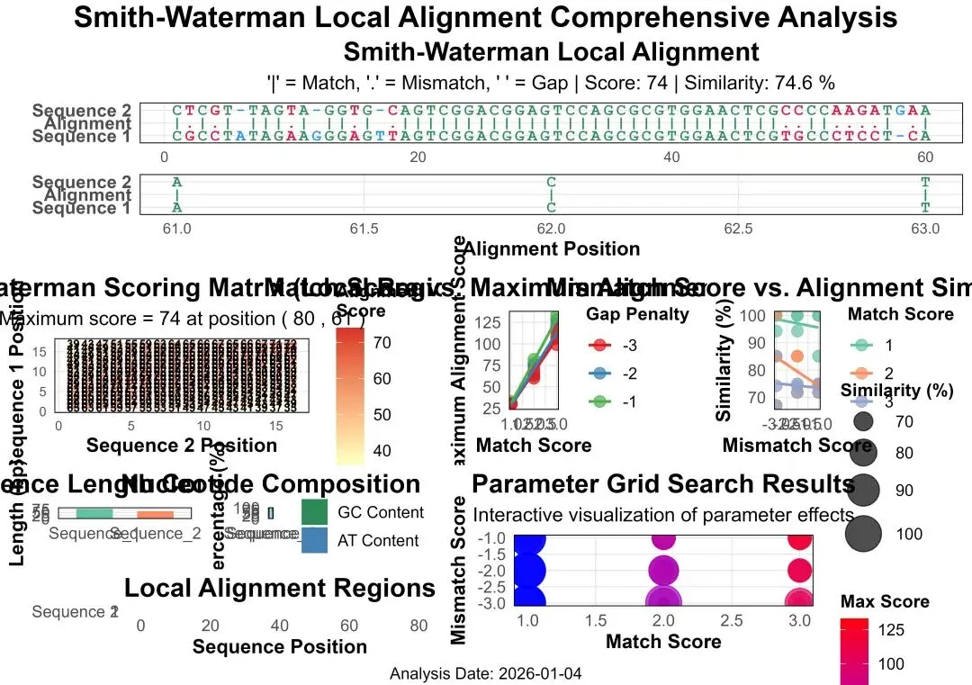
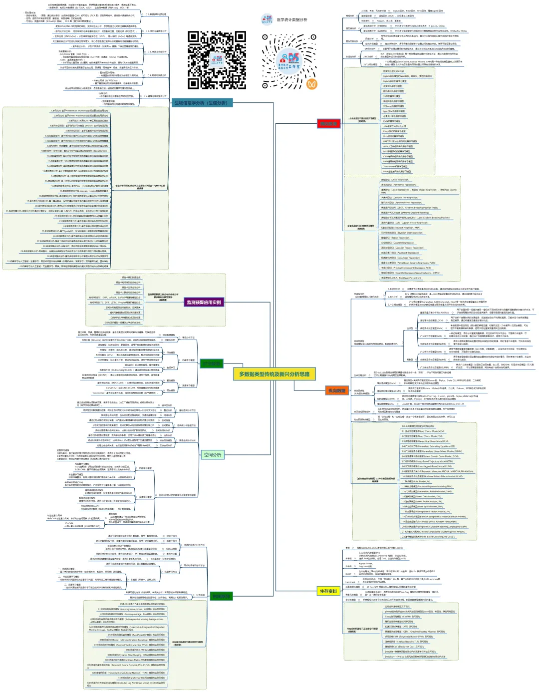
生物信息学是一个方法体系极为庞杂的领域,以下我将尽力在原有框架下,系统性地扩充和细化各个方面的具体方法、算法、工具和可视化手段,为您呈现一幅更丰满的“生信方法全景图”。
1.序列比对-基于Needleman-Wunsch动态规划算法的全局比对
2.序列比对-基于Smith-Waterman动态规划算法的局部比对
3.序列比对-采用BLAST等工具的启发式搜索
4.序列特征识别:基于隐马尔可夫模型(HMM)的序列特征识别
5.序列特征识别:基于权重矩阵的序列特征识别
6.比较基因组学:基于序列比对最大似然法的构建进化树系统发育重建
7.比较基因组学:基于序列比对贝叶斯推断的构建进化树系统发育重建
8.结构分析:同源建模:基于已知结构的同源蛋白预测目标蛋白结构
9.结构分析:分子对接:模拟小分子与蛋白质的相互作用(如AutoDock)
10.功能富集分析-超几何分布检验解读高通量实验筛选出的基因列表
11.功能富集分析-Fisher精确检验解读高通量实验筛选出的基因列表
12.功能富集分析-基因集富集分析解读高通量实验筛选出的基因列表
13.差异表达分析-基于计数模型的RNA-seq数据负二项分布模型统计检验
14.差异表达分析-基于线性模型的转录组数据的基因差异性识别
15.差异表达分析-基于经验贝叶斯模型的转录组数据的基因差异性识别
16.单细胞聚类与注释-使用PCA、t-SNE或UMAP等方法的降维
17.单细胞聚类与注释-Louvain、Leiden等图聚类算法
18.单细胞聚类与注释-通过查找比对已知的细胞类型标记基因定义生物学类型
19.蛋白质互作网络分析-基于基因融合、保守的基因邻接关系的基因组学方法进行网络构建
20.蛋白质互作网络分析-使用MCODE等算法识别紧密连接的功能模块的网络分析
21.系统发育分析-选择压力分析通过计算同义、非同义突变比率(dN/dS)的纯化选择、中性进化还是正选择判断
22.表观遗传学分析-对亚硫酸盐测序数据的DNA甲基化分析
23.表观遗传学分析-基于峰值检测的染色质可及性识别
24.表观遗传学分析-基于峰值检测的蛋白结合分析
25.空间转录组分析-基于SpatialDE、SPARK等统计模型空间变异基因识别
26.空间转录组分析-基于基因表达的空间相似性的空间域识别
27.空间转录组分析-跨多个组织切片的差异空间表达模式多切片比对与差异分析
28.多组学整合分析-关联分析:寻找不同组学层面数据间的统计相关性。
29.多组学整合分析-网络整合:构建包含多类型分子实体及它们之间多层次相互作用的整合网络。
30.多组学整合分析-基于多组学因子分析模型的因子分析与深度学习
31.机器学习与人工智能:监督学习:用已知标签训练分类器(如随机森林、深度学习)预测基因功能、蛋白结构
32.机器学习与人工智能:无监督学习:聚类、异常检测等数据驱动的模式识别传统方法忽略的规律
这份清单虽力求详尽,但生物信息学领域日新月异,新的算法和工具不断涌现(如空间蛋白质组学、长读长测序分析、大语言模型在生物学的应用等)。掌握这些方法的核心思想比记住所有工具名称更重要。在实际研究中,通常需要灵活组合多种方法,形成一条从原始数据到生物学发现的分析流水线。建议的学习路径是:先建立清晰的框架认知(如本回答),然后根据具体研究问题,深入钻研相关的一个或几个子领域。 希望这份扩展版的梳理能为您提供一张有价值的“导航地图”。
医学统计数据分析分享交流SPSS、R语言、Python、ArcGis、Geoda、GraphPad、数据分析图表制作等心得。承接数据分析,论文返修,医学统计,机器学习,生存分析,空间分析,问卷分析,生信分析业务。若有投稿和数据分析代做需求,可以直接联系我,谢谢!

“医学统计数据分析”公众号右下角;
找到“联系作者”,
可加我微信,邀请入粉丝群!

有临床流行病学数据分析
如(t检验、方差分析、χ2检验、logistic回归)、
(重复测量方差分析与配对T检验、ROC曲线)、
(非参数检验、生存分析、样本含量估计)、
(筛检试验:灵敏度、特异度、约登指数等计算)、
(绘制柱状图、散点图、小提琴图、列线图等)、
机器学习、深度学习、生存分析
等需求的同仁们,加入【临床】粉丝群。
疾控,公卫岗位的同仁,可以加一下【公卫】粉丝群,分享生态学研究、空间分析、时间序列、监测数据分析、时空面板技巧等工作科研自动化内容。
有实验室数据分析需求的同仁们,可以加入【生信】粉丝群,交流NCBI(基因序列)、UniProt(蛋白质)、KEGG(通路)、GEO(公共数据集)等公共数据库、基因组学转录组学蛋白组学代谢组学表型组学等数据分析和可视化内容。
或者可扫码直接加微信进群!!!


精品视频课程-“医学统计数据分析”视频号付费合集

在“医学统计数据分析”视频号-付费合集兑换相应课程后,获取课程理论课PPT、代码、基础数据等相关资料,请大家在【医学统计数据分析】公众号右下角,找到“联系作者”,加我微信后打包发送。感谢您的支持!!!
随机文章
-
 10个月宝宝每天需要喝多少奶粉?
- 在 Windows 上跑 Linux,不装双系统、不开虚拟机、不配 SSH.
- 政务年报 PDF 太多不想手抄?用 Python 批量提取表格字段并汇总成 CSV
- 瞬间我对python的兴趣达到了10000 00000%!
- 全部可直接复制运行,这70个Python项目,练完轻松赚外快
- 如何应对供应商涨价和异构Linux环境?现代重工和瑞穗银行都做了同样的选择
- 【案例教程】Python在气象与海洋中的实践技术应用
- 一个基于 PHP 的现代化 B2C 私域电商平台
- ChatGPT第一次跌破50%,Python却越来越稳了
- 【体系教程】基于“python+ADCIRC”潮汐、风驱动循环、风暴潮等海洋水动力模拟;ADCIRC编译安装、前处理和后处理
- 强烈推荐!248页《python编程从入门到实践》完整版,PDF开放下载
