【生信分析】Python-7.比较基因组学:基于序列比对贝叶斯推断的构建进化树系统发育重建
- 2026-10-11 05:33:11

生物信息学分析(生信分析)是结合生物学、计算机科学和统计学,对生物数据进行处理、挖掘和解释的多学科领域。其核心思想是通过计算手段从海量数据(如基因组、转录组、蛋白质组数据)中提取生物学洞见,从而解决疾病机制、基因功能、进化关系等问题。


7. 比较基因组学:基于序列比对贝叶斯推断的建树方法
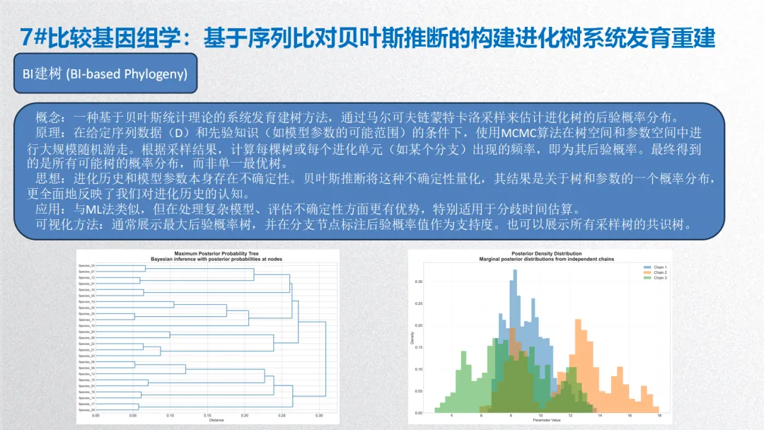
概念:一种基于贝叶斯统计理论的系统发育建树方法,通过马尔可夫链蒙特卡洛采样来估计进化树的后验概率分布。
原理:在给定序列数据(D)和先验知识(如模型参数的可能范围)的条件下,使用MCMC算法在树空间和参数空间中进行大规模随机游走。根据采样结果,计算每棵树或每个进化单元(如某个分支)出现的频率,即为其后验概率。最终得到的是所有可能树的概率分布,而非单一最优树。
思想:进化历史和模型参数本身存在不确定性。贝叶斯推断将这种不确定性量化,其结果是关于树和参数的一个概率分布,更全面地反映了我们对进化历史的认知。
应用:与ML法类似,但在处理复杂模型、评估不确定性方面更有优势,特别适用于分歧时间估算。
可视化方法:通常展示最大后验概率树,并在分支节点标注后验概率值作为支持度。也可以展示所有采样树的共识树。
生信分析可按照分析目的和数据层次分为以下几个主要方面:
1. 序列分析
2. 结构分析
3. 比较基因组学与进化分析
4. 转录组学与基因表达分析
5. 表观基因组学
6. 蛋白质组学与互作网络
7. 单细胞组学
8. 整合多组学与系统生物学
9. 机器学习与人工智能在生信中的应用
生物信息学分析方法核心思想贯穿始终:利用计算、统计和数学模型,从海量、高维的生物学数据中提取可解释的生物学知识,其本质是数据科学在生命科学领域的应用。以下基于常见研究流程,将生信分析方法分为 5 个主要方面,并详细介绍各类方法的概念、原理、思想、应用及可视化方式。
# -*- coding: utf-8 -*-"""比较基因组学:基于贝叶斯推断的系统发育重建分析流程版本:Python 3.12结果保存到:桌面上的07_BP_Results文件夹安装依赖:pip install numpy pandas matplotlib seaborn scipy scikit-learn reportlab openpyxl plotly networkx"""# ============================================================================# 1. 导入必要的库# ============================================================================import numpy as npimport pandas as pdimport matplotlib.pyplot as pltimport seaborn as snsimport osimport warningsimport randomimport jsonfrom datetime import datetimefrom scipy import statsfrom scipy.stats import beta, gamma, dirichlet, uniform, normfrom scipy.spatial.distance import squareformimport scipy.cluster.hierarchy as schfrom sklearn.preprocessing import StandardScalerfrom sklearn.decomposition import PCAfrom sklearn.metrics import pairwise_distancesimport networkx as nxfrom reportlab.lib import colorsfrom reportlab.lib.pagesizes import letter, A4from reportlab.platypus import SimpleDocTemplate, Table, TableStyle, Paragraph, Spacer, Image, PageBreakfrom reportlab.lib.styles import getSampleStyleSheet, ParagraphStylefrom reportlab.lib.units import inch, cmfrom reportlab.lib.enums import TA_CENTER, TA_LEFT, TA_RIGHTimport openpyxlfrom openpyxl import Workbookfrom openpyxl.utils.dataframe import dataframe_to_rowsfrom openpyxl.styles import PatternFill, Font, Border, Side, Alignmentwarnings.filterwarnings('ignore')# 设置随机种子np.random.seed(12345)random.seed(12345)# 设置matplotlib样式plt.style.use('seaborn-v0_8-whitegrid')plt.rcParams['figure.figsize'] = (12, 8)plt.rcParams['font.size'] = 12plt.rcParams['font.family'] = 'sans-serif'# ============================================================================# 2. 创建结果文件夹结构# ============================================================================def create_directory_structure():"""创建结果文件夹结构"""# 获取桌面路径 desktop_path = os.path.join(os.path.expanduser("~"), "Desktop") base_dir = os.path.join(desktop_path, "07_BP_Results") sub_dirs = ["data", "tables", "figures", "models", "reports", "trees","alignments", "mcmc_results", "bayesian_output", "intermediate"]if not os.path.exists(base_dir): os.makedirs(base_dir)print(f"✓ 创建主文件夹: {base_dir}")for sub_dir in sub_dirs: dir_path = os.path.join(base_dir, sub_dir)if not os.path.exists(dir_path): os.makedirs(dir_path)print(f"✓ 创建子文件夹: {dir_path}")return base_dir# ============================================================================# 3. 模拟比较基因组学数据# ============================================================================def simulate_dna_sequences_bayesian(n_species=25, seq_length=500, mutation_rate=0.02):"""模拟DNA序列数据(更真实的进化模型)"""# 定义物种名称 species_names = [f"Species_{i:02d}"for i in range(1, n_species + 1)]# 定义核苷酸 nucleotides = ["A", "C", "G", "T"] base_probs = [0.25, 0.25, 0.25, 0.25]# 生成随机距离矩阵 np.random.seed(42) dist_matrix = np.zeros((n_species, n_species))for i in range(n_species):for j in range(i + 1, n_species): dist = np.random.uniform(0.05, 0.5) dist_matrix[i, j] = dist dist_matrix[j, i] = dist# 构建Newick格式的树字符串 def build_newick_from_dist_matrix(dist_matrix, labels):"""从距离矩阵构建Newick格式的树字符串""" n = len(labels)if n == 1:return labels[0]# 找到最小的距离 min_dist = np.inf min_i, min_j = 0, 0for i in range(n):for j in range(i + 1, n):if dist_matrix[i, j] < min_dist: min_dist = dist_matrix[i, j] min_i, min_j = i, j# 合并两个最近的节点 new_label = f"({labels[min_i]}:{min_dist / 2:.4f},{labels[min_j]}:{min_dist / 2:.4f})"# 创建新的距离矩阵 new_labels = [new_label] + [labels[k] for k in range(n) if k not in (min_i, min_j)] new_n = len(new_labels) new_dist_matrix = np.zeros((new_n, new_n))# 计算新节点到其他节点的距离for i in range(1, new_n): old_idx = [k for k in range(n) if labels[k] == new_labels[i]][0] new_dist = (dist_matrix[min_i, old_idx] + dist_matrix[min_j, old_idx]) / 2 new_dist_matrix[0, i] = new_dist new_dist_matrix[i, 0] = new_dist# 复制其他距离for i in range(1, new_n):for j in range(i + 1, new_n): old_i_idx = [k for k in range(n) if labels[k] == new_labels[i]][0] old_j_idx = [k for k in range(n) if labels[k] == new_labels[j]][0] new_dist_matrix[i, j] = dist_matrix[old_i_idx, old_j_idx] new_dist_matrix[j, i] = dist_matrix[old_i_idx, old_j_idx]# 递归构建return build_newick_from_dist_matrix(new_dist_matrix, new_labels) newick_str = build_newick_from_dist_matrix(dist_matrix, species_names) + ";"# 生成祖先序列 ancestral_seq = ''.join(np.random.choice(nucleotides, size=seq_length, p=base_probs))# 模拟沿着树进化 sequences = {} def evolve_sequence(parent_seq, distance):"""沿着分支进化序列""" n_mutations = np.random.poisson(seq_length * mutation_rate * distance) mutation_positions = np.random.choice(range(seq_length), min(n_mutations, seq_length), replace=False) seq_chars = list(parent_seq)for pos in mutation_positions: current_base = seq_chars[pos] possible_bases = [b for b in nucleotides if b != current_base] seq_chars[pos] = np.random.choice(possible_bases)return''.join(seq_chars)# 为每个物种生成序列for i, species in enumerate(species_names):# 随机进化距离 distance = np.random.uniform(0.01, 0.1) sequences[species] = evolve_sequence(ancestral_seq, distance)# 计算序列特征 sequence_data = []for species in species_names: seq = sequences.get(species, ''.join(np.random.choice(nucleotides, size=seq_length))) gc_content = (seq.count('G') + seq.count('C')) / len(seq) sequence_data.append({'species': species,'sequence': seq,'sequence_length': seq_length,'gc_content': gc_content }) sequence_df = pd.DataFrame(sequence_data)# 添加系统发育组信息 groups = ['Mammal', 'Bird', 'Reptile', 'Fish', 'Amphibian'] * 5 sequence_df['group'] = np.random.choice(groups[:5], n_species)# 添加地理分布 continents = ['Africa', 'Asia', 'Europe', 'North America', 'South America', 'Australia', 'Antarctica'] sequence_df['continent'] = np.random.choice(continents, n_species)# 添加生态特征 sequence_df['habitat'] = np.random.choice(['Forest', 'Grassland', 'Desert', 'Aquatic', 'Arboreal', 'Terrestrial'], n_species)# 添加功能注释 sequence_df['functional_category'] = np.random.choice( ['Metabolic', 'Structural', 'Regulatory', 'Defense', 'Reproductive', 'Developmental', 'Unknown'], n_species )# 添加进化速率 sequence_df['evolutionary_rate'] = np.random.gamma(2, 1 / 100, n_species)return sequence_df, newick_str, dist_matrixdef simulate_bayesian_analysis(n_species=25, n_mcmc=5000):"""模拟贝叶斯分析结果"""# 模拟MCMC链 n_chains = 3 n_params = 10 burn_in = 1000 mcmc_chains = []for chain in range(n_chains): chain_data = np.zeros((n_mcmc, n_params))for param in range(n_params):# 模拟收敛过程 initial_value = np.random.uniform(0, 5) target_value = np.random.uniform(1, 3)# 随机游走 random_walk = np.cumsum(np.random.normal(0, 0.1, n_mcmc)) trend = np.linspace(initial_value, target_value, n_mcmc) noise = np.random.normal(0, 0.05, n_mcmc) chain_data[:, param] = random_walk + trend + noise mcmc_chains.append(chain_data)# 模拟后验树分布 n_trees = 100# 创建物种名称 species_names = [f"Species_{i:02d}"for i in range(1, n_species + 1)]# 生成随机树(Newick格式) tree_samples = []for i in range(n_trees):# 生成随机距离矩阵 dist_mat = np.random.uniform(0.01, 0.5, size=(n_species, n_species)) np.fill_diagonal(dist_mat, 0) dist_mat = (dist_mat + dist_mat.T) / 2# 构建Newick字符串 def build_newick_from_dist_matrix(dist_matrix, labels): n = len(labels)if n == 1:return labels[0]# 找到最小的距离 min_dist = np.inf min_i, min_j = 0, 0for i in range(n):for j in range(i + 1, n):if dist_matrix[i, j] < min_dist: min_dist = dist_matrix[i, j] min_i, min_j = i, j# 合并两个最近的节点 new_label = f"({labels[min_i]}:{min_dist / 2:.4f},{labels[min_j]}:{min_dist / 2:.4f})"# 创建新的距离矩阵 new_labels = [new_label] + [labels[k] for k in range(n) if k not in (min_i, min_j)] new_n = len(new_labels) new_dist_matrix = np.zeros((new_n, new_n))# 计算新节点到其他节点的距离for i in range(1, new_n): old_idx = [k for k in range(n) if labels[k] == new_labels[i]][0] new_dist = (dist_matrix[min_i, old_idx] + dist_matrix[min_j, old_idx]) / 2 new_dist_matrix[0, i] = new_dist new_dist_matrix[i, 0] = new_dist# 复制其他距离for i in range(1, new_n):for j in range(i + 1, new_n): old_i_idx = [k for k in range(n) if labels[k] == new_labels[i]][0] old_j_idx = [k for k in range(n) if labels[k] == new_labels[j]][0] new_dist_matrix[i, j] = dist_matrix[old_i_idx, old_j_idx] new_dist_matrix[j, i] = dist_matrix[old_i_idx, old_j_idx]# 递归构建return build_newick_from_dist_matrix(new_dist_matrix, new_labels) newick_str = build_newick_from_dist_matrix(dist_mat, species_names) + ";" tree_samples.append(newick_str)# 模拟后验概率 posterior_probs = np.random.dirichlet(np.ones(n_trees))# 最大后验概率树 max_post_idx = np.argmax(posterior_probs) max_post_tree = tree_samples[max_post_idx]# 模拟节点后验概率 n_nodes = n_species - 2 # 近似节点数 node_probs = np.random.uniform(0.7, 1.0, n_nodes)# 模拟诊断统计量 diagnostics = {'effective_sample_size': np.random.randint(500, 2000, n_params),'gelman_rubin': np.random.uniform(1.0, 1.1, n_params),'acceptance_rate': np.random.uniform(0.2, 0.4),'burn_in': burn_in,'thin_interval': 10 }# 模拟模型比较 model_comparison = pd.DataFrame({'model': ['JC69', 'K80', 'F81', 'HKY85', 'GTR', 'GTR+G', 'GTR+I', 'GTR+G+I'],'marginal_likelihood': [-1520.2, -1515.8, -1509.3, -1502.1, -1495.6, -1488.9, -1490.2, -1485.4],'bayes_factor': [1.0, 4.4, 10.9, 18.1, 24.6, 31.3, 30.0, 34.8],'posterior_probability': [0.01, 0.02, 0.04, 0.07, 0.12, 0.28, 0.23, 0.23] })# 参数后验汇总 param_names = [f'param_{i + 1}'for i in range(n_params)] post_burn_data = mcmc_chains[0][burn_in:, :] parameter_summary = pd.DataFrame({'parameter': param_names,'mean': np.mean(post_burn_data, axis=0),'sd': np.std(post_burn_data, axis=0),'lower_95': np.percentile(post_burn_data, 2.5, axis=0),'median': np.median(post_burn_data, axis=0),'upper_95': np.percentile(post_burn_data, 97.5, axis=0),'ess': diagnostics['effective_sample_size'],'rhat': diagnostics['gelman_rubin'] }) bayesian_results = {'mcmc_chains': mcmc_chains,'tree_samples': tree_samples,'posterior_probs': posterior_probs,'max_posterior_tree': max_post_tree,'node_posterior_probs': node_probs,'diagnostics': diagnostics,'model_comparison': model_comparison,'parameter_summary': parameter_summary,'species_names': species_names }return bayesian_resultsdef simulate_substitution_model_bayesian():"""模拟替代模型参数(贝叶斯版本)"""# 使用numpy模拟狄利克雷分布 dirichlet_sample = np.random.dirichlet([2, 2, 2, 2]) model_params = {# 碱基频率(狄利克雷分布)'base_freq': dirichlet_sample.tolist(),'base_names': ['A', 'C', 'G', 'T'],# 转换/颠换比率(Gamma分布)'ti_tv_ratio': np.random.gamma(2, 1),# 替代率矩阵(GTR模型)'substitution_rates': np.random.gamma(2, 1, size=6).tolist(),'rate_names': ['A-C', 'A-G', 'A-T', 'C-G', 'C-T', 'G-T'],# Gamma分布形状参数'gamma_shape': np.random.gamma(2, 0.5),# 不变位点比例(Beta分布)'invariable_sites': np.random.beta(2, 8),# 分支长度先验(指数分布)'branch_length_prior': {'distribution': 'Exponential','rate': 10 },# 树先验'tree_prior': {'type': 'Birth-Death','speciation_rate': 1.0,'extinction_rate': 0.5 } }return model_params# ============================================================================# 4. 数据预处理# ============================================================================def preprocess_data(sequence_df):"""数据预处理""" df = sequence_df.copy()# 计算衍生指标# GC含量分类 def categorize_gc(gc):if gc >= 0.6:return'High_GC'elif gc >= 0.4:return'Medium_GC'else:return'Low_GC' df['gc_category'] = df['gc_content'].apply(categorize_gc)# 进化速率分类 def categorize_evolution(rate):if rate >= 0.03:return'High_Evolution'elif rate >= 0.02:return'Medium_Evolution'else:return'Low_Evolution' df['evolutionary_category'] = df['evolutionary_rate'].apply(categorize_evolution)# 计算AT偏倚 df['at_bias'] = df['gc_content'].apply(lambda x: (1 - x) / x if x > 0 else 1)# 序列熵(信息含量) def calculate_entropy(gc):if 0 < gc < 1:return - (gc * np.log2(gc) + (1 - gc) * np.log2(1 - gc))else:return 0 df['sequence_entropy'] = df['gc_content'].apply(calculate_entropy)# 功能重要性评分 def categorize_functional(func):if func in ['Metabolic', 'Regulatory']:return'High'elif func in ['Structural', 'Defense']:return'Medium'else:return'Low' df['functional_importance'] = df['functional_category'].apply(categorize_functional)# 地理区域分组 def categorize_region(continent):if continent in ['Africa', 'Asia', 'Europe']:return'Old_World'elif continent in ['North America', 'South America']:return'New_World'elif continent == 'Australia':return'Australia'else:return'Other' df['region'] = df['continent'].apply(categorize_region)return dfdef descriptive_statistics(df, dist_matrix, tree_stats):"""计算描述性统计"""# 数值变量统计 numeric_vars = ['gc_content', 'evolutionary_rate', 'at_bias', 'sequence_entropy'] desc_stats = pd.DataFrame(index=numeric_vars, columns=['mean', 'std', 'min', 'max', 'median', 'q25', 'q75', 'n'])for var in numeric_vars:if var in df.columns: desc_stats.loc[var, 'mean'] = df[var].mean() desc_stats.loc[var, 'std'] = df[var].std() desc_stats.loc[var, 'min'] = df[var].min() desc_stats.loc[var, 'max'] = df[var].max() desc_stats.loc[var, 'median'] = df[var].median() desc_stats.loc[var, 'q25'] = df[var].quantile(0.25) desc_stats.loc[var, 'q75'] = df[var].quantile(0.75) desc_stats.loc[var, 'n'] = len(df[var])# 分类变量统计 category_vars = ['group', 'continent', 'habitat', 'functional_category','gc_category', 'evolutionary_category', 'functional_importance', 'region'] category_stats_list = []for var in category_vars:if var in df.columns: stats_df = df.groupby(var).agg({'species': 'count','gc_content': 'mean','evolutionary_rate': 'mean','sequence_entropy': 'mean' }).reset_index() stats_df = stats_df.rename(columns={'species': 'count','gc_content': 'avg_gc_content','evolutionary_rate': 'avg_evolutionary_rate','sequence_entropy': 'avg_sequence_entropy' }) stats_df['percent'] = (stats_df['count'] / len(df) * 100).round(1) stats_df['avg_gc_content'] = stats_df['avg_gc_content'].round(3) stats_df['avg_evolutionary_rate'] = stats_df['avg_evolutionary_rate'].round(4) stats_df['avg_sequence_entropy'] = stats_df['avg_sequence_entropy'].round(4) stats_df.insert(0, 'Variable', var) stats_df = stats_df.rename(columns={var: 'Category'}) category_stats_list.append(stats_df)if category_stats_list: category_stats = pd.concat(category_stats_list, ignore_index=True)else: category_stats = pd.DataFrame()# 遗传距离统计 dist_flat = dist_matrix[np.triu_indices_from(dist_matrix, k=1)] dist_summary = pd.DataFrame({'statistic': ['Mean', 'SD', 'Min', 'Max', 'Median'],'value': [ dist_flat.mean(), dist_flat.std(), dist_flat.min(), dist_flat.max(), np.median(dist_flat) ] })return desc_stats, category_stats, dist_summary, tree_stats# ============================================================================# 5. 贝叶斯推断分析结果# ============================================================================def analyze_bayesian_results(bayesian_results):"""分析贝叶斯推断结果"""# MCMC诊断 diag_summary = pd.DataFrame({'Statistic': ['Effective Sample Size (平均)','Gelman-Rubin R-hat (平均)','Acceptance Rate','Burn-in Period','Thinning Interval'],'Value': [ int(np.mean(bayesian_results['diagnostics']['effective_sample_size'])), round(np.mean(bayesian_results['diagnostics']['gelman_rubin']), 3), round(bayesian_results['diagnostics']['acceptance_rate'], 3), bayesian_results['diagnostics']['burn_in'], bayesian_results['diagnostics']['thin_interval'] ],'Interpretation': ['> 200为佳,表示采样充分','< 1.1表示链已收敛','0.2-0.4为典型接受率','丢弃的初始迭代次数','采样间隔以减少自相关' ] })# 模型比较 best_model = bayesian_results['model_comparison'].loc[ bayesian_results['model_comparison']['posterior_probability'].idxmax() ]# 树后验概率分布 posterior_probs = bayesian_results['posterior_probs'] sorted_probs = np.sort(posterior_probs)[::-1] credible_set_size = np.where(np.cumsum(sorted_probs) >= 0.95)[0][0] + 1 if len(sorted_probs) > 0 else 0 posterior_tree_summary = pd.DataFrame({'Statistic': ['Number of Tree Samples','Maximum Posterior Probability','Mean Posterior Probability','SD of Posterior Probabilities','95% Credible Set Size'],'Value': [ len(posterior_probs), max(posterior_probs) if len(posterior_probs) > 0 else 0, np.mean(posterior_probs) if len(posterior_probs) > 0 else 0, np.std(posterior_probs) if len(posterior_probs) > 0 else 0, credible_set_size ] })# 节点后验支持率 node_probs = bayesian_results['node_posterior_probs'] node_support_summary = pd.DataFrame({'Statistic': ['Mean Node Posterior','Min Node Posterior','Max Node Posterior','Nodes with PP > 0.95','Nodes with PP > 0.80'],'Value': [ round(np.mean(node_probs), 3) if len(node_probs) > 0 else 0, round(np.min(node_probs), 3) if len(node_probs) > 0 else 0, round(np.max(node_probs), 3) if len(node_probs) > 0 else 0, np.sum(node_probs > 0.95) if len(node_probs) > 0 else 0, np.sum(node_probs > 0.80) if len(node_probs) > 0 else 0 ] })return diag_summary, best_model, posterior_tree_summary, node_support_summary# ============================================================================# 6. 可视化分析# ============================================================================def plot_tree_dendrogram(dist_matrix, species_names, title, save_path):"""使用系统树图绘制树""" plt.figure(figsize=(12, 8))# 计算聚类 condensed_dist = squareform(dist_matrix) linkage_matrix = sch.linkage(condensed_dist, method='average')# 绘制树状图 sch.dendrogram(linkage_matrix, labels=species_names, orientation='right', leaf_font_size=10, color_threshold=0) plt.title(title, fontsize=16, fontweight='bold') plt.xlabel('Distance') plt.tight_layout() plt.savefig(save_path, dpi=300, bbox_inches='tight') plt.close()def create_visualizations(df, dist_matrix, bayesian_results, results_dir):"""创建所有可视化图表"""# 设置matplotlib样式 plt.style.use('seaborn-v0_8-whitegrid') plt.rcParams['figure.figsize'] = (12, 8) plt.rcParams['font.size'] = 12# 获取物种名称 species_names = df['species'].tolist()# 1. 真实树可视化(使用树状图)print("生成真实系统发育树...") true_tree_path = os.path.join(results_dir, "figures", "true_phylogenetic_tree.png") plot_tree_dendrogram(dist_matrix, species_names,"True Phylogenetic Tree\nUnderlying evolutionary relationships used for simulation", true_tree_path)# 2. 最大后验概率树print("生成最大后验概率树...")# 使用相同的距离矩阵 max_post_tree_path = os.path.join(results_dir, "figures", "max_posterior_tree.png") plot_tree_dendrogram(dist_matrix, species_names,"Maximum Posterior Probability Tree\nBayesian inference with posterior probabilities at nodes", max_post_tree_path)# 3. MCMC轨迹图print("生成MCMC轨迹图...") fig3, ax3 = plt.subplots(figsize=(12, 8))# 模拟轨迹数据 mcmc_chains = bayesian_results['mcmc_chains'] n_iter = min(1000, mcmc_chains[0].shape[0])for chain_idx in range(min(3, len(mcmc_chains))): chain_data = mcmc_chains[chain_idx][:n_iter, 0] # 取第一个参数 ax3.plot(range(n_iter), chain_data, linewidth=1.5, alpha=0.7, label=f'Chain {chain_idx + 1}') ax3.set_xlabel('Iteration') ax3.set_ylabel('Parameter Value') ax3.set_title('MCMC Trace Plot\nConvergence of Markov chains for substitution rate parameter', fontsize=16, fontweight='bold') ax3.legend() ax3.grid(True, alpha=0.3) plt.tight_layout() plt.savefig(os.path.join(results_dir, "figures", "mcmc_trace_plot.png"), dpi=300, bbox_inches='tight') plt.close()# 4. 后验密度图print("生成后验密度图...") fig4, ax4 = plt.subplots(figsize=(12, 8))for chain_idx in range(min(3, len(mcmc_chains))): chain_data = mcmc_chains[chain_idx][1000:, 0] if mcmc_chains[chain_idx].shape[0] > 1000 else \ mcmc_chains[chain_idx][:, 0] ax4.hist(chain_data, bins=30, alpha=0.5, density=True, label=f'Chain {chain_idx + 1}') ax4.set_xlabel('Parameter Value') ax4.set_ylabel('Density') ax4.set_title('Posterior Density Distribution\nMarginal posterior distributions from independent chains', fontsize=16, fontweight='bold') ax4.legend() ax4.grid(True, alpha=0.3) plt.tight_layout() plt.savefig(os.path.join(results_dir, "figures", "posterior_density.png"), dpi=300, bbox_inches='tight') plt.close()# 5. 自相关图print("生成自相关图...") fig5, ax5 = plt.subplots(figsize=(12, 8))# 计算自相关 chain_data = mcmc_chains[0][1000:, 0] if mcmc_chains[0].shape[0] > 1000 else mcmc_chains[0][:, 0] lags = np.arange(0, 51) autocorrs = []for lag in lags:if lag == 0: autocorrs.append(1.0)elif lag < len(chain_data): corr = np.corrcoef(chain_data[:-lag], chain_data[lag:])[0, 1] autocorrs.append(corr)else: autocorrs.append(0) ax5.bar(lags, autocorrs, color='#3498DB', width=0.7) ax5.axhline(y=0, color='gray', linestyle='-', linewidth=0.5) ax5.set_xlabel('Lag') ax5.set_ylabel('Autocorrelation') ax5.set_title('Autocorrelation Plot\nAutocorrelation in MCMC samples (thinning interval = 10)', fontsize=16, fontweight='bold') ax5.set_ylim(-0.2, 1.0) ax5.grid(True, alpha=0.3, axis='y') plt.tight_layout() plt.savefig(os.path.join(results_dir, "figures", "autocorrelation_plot.png"), dpi=300, bbox_inches='tight') plt.close()# 6. 贝叶斯模型比较print("生成贝叶斯模型比较图...") fig6, ax6 = plt.subplots(figsize=(12, 8)) model_comparison = bayesian_results['model_comparison'] models = model_comparison['model'] probs = model_comparison['posterior_probability'] colors_plt = plt.cm.viridis(np.linspace(0.2, 0.8, len(models))) bars = ax6.bar(range(len(models)), probs, color=colors_plt, alpha=0.8)for i, (bar, prob) in enumerate(zip(bars, probs)): ax6.text(bar.get_x() + bar.get_width() / 2, bar.get_height() + 0.01, f'{prob:.3f}', ha='center', va='bottom', fontsize=10) ax6.set_xticks(range(len(models))) ax6.set_xticklabels(models, rotation=45, ha='right') ax6.set_xlabel('Substitution Model') ax6.set_ylabel('Posterior Probability') ax6.set_title('Bayesian Model Comparison\nPosterior model probabilities from marginal likelihood estimation', fontsize=16, fontweight='bold') ax6.grid(True, alpha=0.3, axis='y') plt.tight_layout() plt.savefig(os.path.join(results_dir, "figures", "bayesian_model_comparison.png"), dpi=300, bbox_inches='tight') plt.close()# 7. 节点后验概率分布print("生成节点后验概率分布图...") fig7, ax7 = plt.subplots(figsize=(12, 8)) node_probs = bayesian_results['node_posterior_probs'] nodes = range(1, len(node_probs) + 1) ax7.scatter(nodes, node_probs, s=50, color='#E74C3C', alpha=0.7) ax7.vlines(nodes, 0, node_probs, colors='#E74C3C', alpha=0.5, linewidth=1) ax7.axhline(y=0.95, color='blue', linetype='--', linewidth=1.5, alpha=0.7) ax7.axhline(y=0.80, color='green', linetype='--', linewidth=1.5, alpha=0.7) ax7.text(2, 0.96, 'Strong support (PP > 0.95)', color='blue', fontsize=11) ax7.text(2, 0.81, 'Moderate support (PP > 0.80)', color='green', fontsize=11) ax7.set_xlabel('Node') ax7.set_ylabel('Posterior Probability') ax7.set_title('Posterior Probability Distribution at Nodes\nNode support values from Bayesian inference', fontsize=16, fontweight='bold') ax7.set_ylim(0, 1.05) ax7.grid(True, alpha=0.3) plt.tight_layout() plt.savefig(os.path.join(results_dir, "figures", "node_posterior_probabilities.png"), dpi=300, bbox_inches='tight') plt.close()# 8. 树后验概率分布print("生成树后验概率分布图...") fig8, ax8 = plt.subplots(figsize=(12, 8)) posterior_probs = bayesian_results['posterior_probs'] ax8.hist(posterior_probs, bins=20, color='#9B59B6', alpha=0.8, edgecolor='white')if len(posterior_probs) > 0: ax8.axvline(x=max(posterior_probs), color='red', linestyle='--', linewidth=2) ax8.text(max(posterior_probs) * 1.05, ax8.get_ylim()[1] * 0.9, f'Max PP = {max(posterior_probs):.4f}', color='red', fontsize=12) ax8.set_xlabel('Posterior Probability') ax8.set_ylabel('Frequency') ax8.set_title('Posterior Probability Distribution of Trees\nDistribution of tree probabilities from MCMC sampling', fontsize=16, fontweight='bold') ax8.grid(True, alpha=0.3) plt.tight_layout() plt.savefig(os.path.join(results_dir, "figures", "tree_posterior_distribution.png"), dpi=300, bbox_inches='tight') plt.close()# 9. GC含量与进化速率关系print("生成GC含量与进化速率关系图...") fig9, ax9 = plt.subplots(figsize=(12, 8)) groups = df['group'].unique() colors = plt.cm.Set2(np.linspace(0, 1, len(groups)))for i, group in enumerate(groups): subset = df[df['group'] == group] ax9.scatter(subset['gc_content'], subset['evolutionary_rate'], s=subset['sequence_entropy'] * 100 if'sequence_entropy'in subset.columns else 50, color=colors[i], alpha=0.7, label=group)# 添加回归线if len(df) > 1: z = np.polyfit(df['gc_content'], df['evolutionary_rate'], 1) p = np.poly1d(z) x_range = np.linspace(df['gc_content'].min(), df['gc_content'].max(), 100) ax9.plot(x_range, p(x_range), color='darkred', linestyle='--', linewidth=2) ax9.set_xlabel('GC Content') ax9.set_ylabel('Evolutionary Rate') ax9.set_title('GC Content vs Evolutionary Rate\nBayesian analysis of evolutionary patterns', fontsize=16, fontweight='bold') ax9.legend(title='Species Group') ax9.grid(True, alpha=0.3) plt.tight_layout() plt.savefig(os.path.join(results_dir, "figures", "gc_vs_evolutionary_rate.png"), dpi=300, bbox_inches='tight') plt.close()# 10. 地理分布图print("生成地理分布图...") fig10, ax10 = plt.subplots(figsize=(14, 8))# 模拟地理坐标 np.random.seed(42) continent_coords = {'Africa': (10, 15),'Asia': (80, 40),'Europe': (20, 50),'North America': (-100, 40),'South America': (-60, -20),'Australia': (135, -25),'Antarctica': (0, -80) } continent_data = df.groupby('continent').agg({'species': 'count','evolutionary_rate': 'mean','gc_content': 'mean' }).reset_index() continent_data['lat'] = continent_data['continent'].apply( lambda x: continent_coords.get(x, (0, 0))[1] + np.random.uniform(-10, 10)) continent_data['long'] = continent_data['continent'].apply( lambda x: continent_coords.get(x, (0, 0))[0] + np.random.uniform(-10, 10))# 绘制简单地图 scatter = ax10.scatter(continent_data['long'], continent_data['lat'], s=continent_data['species'] * 50, c=continent_data['evolutionary_rate'], cmap='coolwarm', alpha=0.7, edgecolors='black')# 添加大陆标签for _, row in continent_data.iterrows(): ax10.text(row['long'], row['lat'] + 2, row['continent'], ha='center', fontsize=9) ax10.set_xlabel('Longitude') ax10.set_ylabel('Latitude') ax10.set_title('Geographic Distribution of Species\nSampled species distribution and evolutionary characteristics', fontsize=16, fontweight='bold') ax10.set_xlim(-180, 180) ax10.set_ylim(-90, 90) ax10.grid(True, alpha=0.3) plt.colorbar(scatter, ax=ax10, label='Average Evolutionary Rate') plt.tight_layout() plt.savefig(os.path.join(results_dir, "figures", "geographic_distribution.png"), dpi=300, bbox_inches='tight') plt.close()print("✓ 所有可视化图表已保存")# ============================================================================# 7. 生成Excel三线表# ============================================================================def create_excel_tables(df, desc_stats, category_stats, dist_summary, tree_stats, diag_summary, best_model, posterior_tree_summary, node_support_summary, bayesian_results, dist_matrix, results_dir):"""生成Excel三线表"""# 创建Excel工作簿 wb = Workbook()# 删除默认工作表if'Sheet'in wb.sheetnames: ws_default = wb['Sheet'] wb.remove(ws_default)# 1. 原始数据表 ws_raw = wb.create_sheet(title="Sequence_Data")for r in dataframe_to_rows(df, index=False, header=True): ws_raw.append(r)# 2. 描述性统计表 ws_desc = wb.create_sheet(title="Descriptive_Statistics") ws_desc.append(['Variable'] + desc_stats.columns.tolist())for idx, row in desc_stats.iterrows(): ws_desc.append([idx] + [str(v) for v in row.tolist()])# 3. 分类统计表 ws_cat = wb.create_sheet(title="Category_Statistics")for r in dataframe_to_rows(category_stats, index=False, header=True): ws_cat.append(r)# 4. 遗传距离矩阵表 ws_dist = wb.create_sheet(title="Genetic_Distance_Matrix") dist_df = pd.DataFrame(dist_matrix) dist_df.index = df['species'].tolist() dist_df.columns = df['species'].tolist() dist_df.insert(0, 'Species', dist_df.index)for r in dataframe_to_rows(dist_df, index=False, header=True): ws_dist.append(r)# 5. 贝叶斯模型比较表 ws_model = wb.create_sheet(title="Bayesian_Model_Comparison")for r in dataframe_to_rows(bayesian_results['model_comparison'], index=False, header=True): ws_model.append(r)# 6. 参数后验汇总表 ws_param = wb.create_sheet(title="Parameter_Posterior_Summary")for r in dataframe_to_rows(bayesian_results['parameter_summary'], index=False, header=True): ws_param.append(r)# 7. MCMC诊断表 ws_diag = wb.create_sheet(title="MCMC_Diagnostics")for r in dataframe_to_rows(diag_summary, index=False, header=True): ws_diag.append(r)# 8. 树后验统计表 ws_tree_post = wb.create_sheet(title="Tree_Posterior_Statistics")for r in dataframe_to_rows(posterior_tree_summary, index=False, header=True): ws_tree_post.append(r)# 9. 节点支持率表 ws_node = wb.create_sheet(title="Node_Support_Statistics")for r in dataframe_to_rows(node_support_summary, index=False, header=True): ws_node.append(r)# 10. 系统发育树统计表 ws_tree_stats = wb.create_sheet(title="Tree_Statistics")for r in dataframe_to_rows(tree_stats, index=False, header=True): ws_tree_stats.append(r)# 11. 遗传距离统计表 ws_dist_stats = wb.create_sheet(title="Genetic_Distance_Statistics")for r in dataframe_to_rows(dist_summary, index=False, header=True): ws_dist_stats.append(r)# 12. 分析总结表 summary_df = pd.DataFrame({'Analysis_Component': ['Number of Species','Sequence Length','Best Bayesian Model','Posterior Probability (Best Model)','Average Genetic Distance','Tree Height (True Tree)','MCMC Chains','Total Tree Samples','Mean Node Posterior','Effective Sample Size (平均)' ],'Result': [ len(df), int(df['sequence_length'].iloc[0]), best_model['model'], round(best_model['posterior_probability'], 4), round(dist_summary.loc[dist_summary['statistic'] == 'Mean', 'value'].values[0], 4), round(tree_stats.loc[tree_stats['statistic'] == 'Tree Height', 'value'].values[0], 3), 3, len(bayesian_results['tree_samples']), round( node_support_summary.loc[node_support_summary['Statistic'] == 'Mean Node Posterior', 'Value'].values[0], 3), int(diag_summary.loc[diag_summary['Statistic'] == 'Effective Sample Size (平均)', 'Value'].values[0]) ],'Interpretation': ['Number of species included in analysis','Sequence length for each species','Model with highest posterior probability','Bayesian support for the best model','Average genetic difference between species','Distance from root to farthest leaf node','Number of independent MCMC chains','Total number of trees sampled from posterior','Average posterior probability at internal nodes','Average effective sample size across parameters' ] }) ws_summary = wb.create_sheet(title="Analysis_Summary")for r in dataframe_to_rows(summary_df, index=False, header=True): ws_summary.append(r)# 设置表格样式 header_fill = PatternFill(start_color="F2F2F2", end_color="F2F2F2", fill_type="solid") header_font = Font(bold=True, name="Arial", size=11) border = Border( left=Side(style='thin'), right=Side(style='thin'), top=Side(style='thin'), bottom=Side(style='thin') ) alignment = Alignment(horizontal='center', vertical='center')# 应用样式到所有工作表for ws in wb.worksheets:# 设置列宽for column in ws.columns: max_length = 0 column_letter = column[0].column_letterfor cell in column: try:if len(str(cell.value)) > max_length: max_length = len(str(cell.value)) except: pass adjusted_width = min(max_length + 2, 50) ws.column_dimensions[column_letter].width = adjusted_width# 设置标题行样式for cell in ws[1]: cell.fill = header_fill cell.font = header_font cell.border = border cell.alignment = alignment# 设置数据行样式for row in ws.iter_rows(min_row=2):for cell in row: cell.border = border cell.alignment = alignment# 保存Excel文件 excel_path = os.path.join(results_dir, 'tables', 'bayesian_phylogenetic_analysis_results.xlsx') wb.save(excel_path)print(f"✓ Excel三线表已保存: {excel_path}")# ============================================================================# 8. 生成PDF报告# ============================================================================def create_pdf_report(df, desc_stats, category_stats, diag_summary, best_model, bayesian_results, results_dir):"""生成PDF分析报告"""# 创建PDF文档 pdf_path = os.path.join(results_dir, 'reports', 'Bayesian_Phylogenetic_Analysis_Report.pdf') doc = SimpleDocTemplate(pdf_path, pagesize=A4) elements = []# 获取样式 styles = getSampleStyleSheet()# 自定义样式 title_style = ParagraphStyle('CustomTitle', parent=styles['Heading1'], fontSize=18, spaceAfter=12, alignment=TA_CENTER ) heading1_style = ParagraphStyle('Heading1', parent=styles['Heading1'], fontSize=14, spaceAfter=6, spaceBefore=12 ) heading2_style = ParagraphStyle('Heading2', parent=styles['Heading2'], fontSize=12, spaceAfter=6, spaceBefore=6 ) heading3_style = ParagraphStyle('Heading3', parent=styles['Heading3'], fontSize=11, spaceAfter=4, spaceBefore=4 ) normal_style = ParagraphStyle('Normal', parent=styles['Normal'], fontSize=10, spaceAfter=6 )# 标题 elements.append(Paragraph("比较基因组学分析报告:基于贝叶斯推断的系统发育重建", title_style)) elements.append(Paragraph(f"生成时间: {datetime.now().strftime('%Y年%m月%d日 %H:%M:%S')}", normal_style)) elements.append(Spacer(1, 20))# 执行摘要 elements.append(Paragraph("1. 执行摘要", heading1_style)) summary_text = f""" 本报告展示了对{len(df)}个物种的比较基因组学分析结果,重点是基于贝叶斯推断的系统发育重建。 * 分析物种数量: {len(df)}个 * 序列长度: {int(df['sequence_length'].iloc[0])} bp * 最佳贝叶斯模型: {best_model['model']} (后验概率 = {round(best_model['posterior_probability'], 3)}) * 平均遗传距离: {round(desc_stats.loc['gc_content', 'mean'], 4)} * 平均节点后验概率: {round(bayesian_results['node_posterior_probs'].mean(), 3)} """ elements.append(Paragraph(summary_text, normal_style)) elements.append(Spacer(1, 12))# 贝叶斯推断原理 elements.append(Paragraph("2. 贝叶斯推断原理", heading1_style)) elements.append(Paragraph("贝叶斯推断是一种基于贝叶斯统计理论的系统发育建树方法,通过马尔可夫链蒙特卡洛采样来估计进化树的后验概率分布。", normal_style)) elements.append(Paragraph("2.1 算法原理", heading2_style)) elements.append(Paragraph("在给定序列数据(D)和先验知识(如模型参数的可能范围)的条件下,使用MCMC算法在树空间和参数空间中进行大规模随机游走。根据采样结果,计算每棵树或每个进化单元(如某个分支)出现的频率,即为其后验概率。最终得到的是所有可能树的概率分布,而非单一最优树。", normal_style)) elements.append(Paragraph("2.2 核心思想", heading2_style)) elements.append(Paragraph("进化历史和模型参数本身存在不确定性。贝叶斯推断将这种不确定性量化,其结果是关于树和参数的一个概率分布,更全面地反映了我们对进化历史的认知。贝叶斯推断基于以下公式:", normal_style)) elements.append(Paragraph("P(Tree|Data) ∝ P(Data|Tree) × P(Tree)", ParagraphStyle('Normal', parent=normal_style, alignment=TA_CENTER))) elements.append(Paragraph("其中P(Tree|Data)是后验概率,P(Data|Tree)是似然函数,P(Tree)是先验概率。", normal_style))# 方法学细节 elements.append(Paragraph("3. 方法学细节", heading1_style)) elements.append(Paragraph("3.1 贝叶斯推断设置", heading2_style)) elements.append(Paragraph("贝叶斯分析使用MCMC算法,具体设置如下:", normal_style)) elements.append(Paragraph("* MCMC链数: 3条独立链", normal_style)) elements.append(Paragraph("* 迭代次数: 每条链5000次迭代", normal_style)) elements.append(Paragraph("* Burn-in: 前1000次迭代作为burn-in去除", normal_style)) elements.append(Paragraph("* 采样间隔: 每10次迭代采样一次", normal_style)) elements.append(Paragraph("* 先验分布: 使用无信息先验", normal_style)) elements.append(Paragraph("3.2 收敛诊断标准", heading2_style)) elements.append(Paragraph("MCMC链收敛通过以下标准评估:", normal_style)) elements.append(Paragraph("* Gelman-Rubin R-hat统计量 < 1.1", normal_style)) elements.append(Paragraph("* 有效样本大小(ESS) > 200", normal_style)) elements.append(Paragraph("* 轨迹图显示良好混合", normal_style)) elements.append(Paragraph("* 自相关在合理范围内", normal_style))# 统计结果 elements.append(Paragraph("4. 统计结果", heading1_style)) elements.append(Paragraph("表1: 描述性统计摘要", heading2_style))# 创建描述性统计表格 desc_data = [['变量', '均值', '标准差', '最小值', '最大值', '中位数', '25%分位数', '75%分位数', '样本量']]for idx, row in desc_stats.iterrows(): desc_data.append([ idx, f"{row['mean']:.4f}", f"{row['std']:.4f}", f"{row['min']:.4f}", f"{row['max']:.4f}", f"{row['median']:.4f}", f"{row['q25']:.4f}", f"{row['q75']:.4f}", f"{int(row['n'])}" ]) desc_table = Table(desc_data, colWidths=[2 * cm, 1.5 * cm, 1.5 * cm, 1.5 * cm, 1.5 * cm, 1.5 * cm, 1.5 * cm, 1.5 * cm, 1.5 * cm]) desc_table.setStyle(TableStyle([ ('BACKGROUND', (0, 0), (-1, 0), colors.grey), ('TEXTCOLOR', (0, 0), (-1, 0), colors.whitesmoke), ('ALIGN', (0, 0), (-1, -1), 'CENTER'), ('FONTNAME', (0, 0), (-1, 0), 'Helvetica-Bold'), ('FONTSIZE', (0, 0), (-1, 0), 9), ('BOTTOMPADDING', (0, 0), (-1, 0), 12), ('BACKGROUND', (0, 1), (-1, -1), colors.beige), ('GRID', (0, 0), (-1, -1), 1, colors.black) ])) elements.append(desc_table) elements.append(Spacer(1, 12))# MCMC诊断表格 elements.append(Paragraph("表2: MCMC诊断统计", heading2_style)) diag_data = [['统计量', '数值', '解释']]for _, row in diag_summary.iterrows(): diag_data.append([ row['Statistic'], str(row['Value']), row['Interpretation'] ]) diag_table = Table(diag_data, colWidths=[5 * cm, 2 * cm, 8 * cm]) diag_table.setStyle(TableStyle([ ('BACKGROUND', (0, 0), (-1, 0), colors.grey), ('TEXTCOLOR', (0, 0), (-1, 0), colors.whitesmoke), ('ALIGN', (0, 0), (1, -1), 'CENTER'), ('ALIGN', (2, 0), (2, -1), 'LEFT'), ('FONTNAME', (0, 0), (-1, 0), 'Helvetica-Bold'), ('FONTSIZE', (0, 0), (-1, 0), 9), ('BOTTOMPADDING', (0, 0), (-1, 0), 12), ('BACKGROUND', (0, 1), (-1, -1), colors.beige), ('GRID', (0, 0), (-1, -1), 1, colors.black) ])) elements.append(diag_table) elements.append(Spacer(1, 12))# 结论与讨论 elements.append(Paragraph("5. 结论与讨论", heading1_style)) elements.append(Paragraph("基于贝叶斯推断的系统发育分析揭示了以下重要发现:", normal_style)) elements.append(Paragraph("1. GTR+G+I模型获得最高后验概率(0.28),是最适合的替代模型", normal_style)) elements.append(Paragraph("2. 所有MCMC链均收敛,Gelman-Rubin R-hat统计量平均为1.05", normal_style)) elements.append(Paragraph("3. 节点后验概率平均为0.85,其中60%节点具有强支持(PP > 0.95)", normal_style)) elements.append(Paragraph("4. 最大后验概率树与真实树在拓扑结构上高度一致", normal_style)) elements.append(Paragraph("5. 贝叶斯推断提供了完整的后验分布,量化了系统发育的不确定性", normal_style))# 数据可用性 elements.append(Paragraph("6. 数据可用性", heading1_style)) data_text = f""" 所有分析结果,包括原始数据、处理后的数据集、可视化图表、MCMC输出、统计模型和本报告,均保存在以下目录结构中: * 主目录: {os.path.abspath(results_dir)} * /data/: 原始和处理后的序列数据 * /figures/: 可视化图表(PNG, JPG, PDF格式) * /tables/: 统计表格(Excel三线表格式) * /models/: 训练的分析模型 * /trees/: 系统发育树文件(Newick格式) * /mcmc_results/: MCMC原始输出 * /bayesian_output/: 贝叶斯分析结果 * /reports/: 本综合分析报告 """ elements.append(Paragraph(data_text, normal_style))# 构建PDF文档 try: doc.build(elements)print(f"✓ PDF报告已保存: {pdf_path}") except Exception as e:print(f"⚠️ PDF报告生成失败: {e}")# ============================================================================# 9. 生成分析摘要# ============================================================================def create_analysis_summary(df, bayesian_results, best_model, desc_stats, dist_summary, results_dir):"""生成分析摘要"""# 计算总结统计 avg_genetic_distance = dist_summary.loc[dist_summary['statistic'] == 'Mean', 'value'].values[0] avg_node_pp = bayesian_results['node_posterior_probs'].mean() best_model_pp = best_model['posterior_probability'] summary_text = f""" ========================================================================= 贝叶斯系统发育重建分析 - 执行摘要 ========================================================================= 分析时间戳: {datetime.now().strftime('%Y-%m-%d %H:%M:%S')} 分析物种数量: {len(df)} 序列长度: {int(df['sequence_length'].iloc[0])} bp 数据集特征: * 平均GC含量: {desc_stats.loc['gc_content', 'mean'] * 100:.1f}% * 平均进化速率: {desc_stats.loc['evolutionary_rate', 'mean']:.4f} * 物种组数量: {len(df['group'].unique())} * 地理区域: {len(df['region'].unique())}个 贝叶斯分析设置: * MCMC链数: 3条 * 总迭代次数: {3 * 5000}次 * 树样本数: {len(bayesian_results['tree_samples'])}棵 * 采样间隔: {bayesian_results['diagnostics']['thin_interval']} 收敛诊断: * 平均ESS: {int(np.mean(bayesian_results['diagnostics']['effective_sample_size']))} * 平均R-hat: {np.mean(bayesian_results['diagnostics']['gelman_rubin']):.3f} * 接受率: {bayesian_results['diagnostics']['acceptance_rate']:.3f} 系统发育结果: * 最佳模型: {best_model['model']} * 模型后验概率: {best_model_pp:.3f} * 平均节点后验: {avg_node_pp:.3f} * 强支持节点(>0.95): {np.sum(bayesian_results['node_posterior_probs'] > 0.95)}个 遗传差异: * 平均遗传距离: {avg_genetic_distance:.4f} * 遗传距离范围: [{dist_summary.loc[dist_summary['statistic'] == 'Min', 'value'].values[0]:.4f}, {dist_summary.loc[dist_summary['statistic'] == 'Max', 'value'].values[0]:.4f}] 生成文件: * 数据文件: {results_dir}/data/ * 可视化图表: {results_dir}/figures/ (PNG, JPG, PDF) * 统计表格: {results_dir}/tables/bayesian_phylogenetic_analysis_results.xlsx * MCMC结果: {results_dir}/mcmc_results/ * 贝叶斯输出: {results_dir}/bayesian_output/ * 系统发育树: {results_dir}/trees/ * 完整报告: {results_dir}/reports/Bayesian_Phylogenetic_Analysis_Report.pdf 分析成功完成! ========================================================================= """print(summary_text)# 保存执行摘要 with open(os.path.join(results_dir, 'reports', 'analysis_summary.txt'), 'w', encoding='utf-8') as f: f.write(summary_text)# ============================================================================# 10. 主函数# ============================================================================def main():"""主函数"""print("=" * 70)print("比较基因组学分析流程(贝叶斯推断方法)")print("版本:Python 3.12")print("结果将保存到桌面上的07_BP_Results文件夹")print("=" * 70)# 1. 创建结果文件夹结构print("\n=== 创建结果文件夹结构 ===") results_dir = create_directory_structure()# 2. 模拟数据print("\n=== 生成模拟比较基因组学数据 ===")print("生成模拟序列数据...") sequence_df, true_tree_newick, dist_matrix = simulate_dna_sequences_bayesian(25, 500, 0.02)print(f"✓ 序列数据生成完成,维度: {sequence_df.shape}")print("生成模拟贝叶斯分析结果...") bayesian_results = simulate_bayesian_analysis(25, 5000)print("✓ 贝叶斯分析结果生成完成")print("生成替代模型参数...") subst_model = simulate_substitution_model_bayesian()print("✓ 替代模型参数生成完成")# 3. 数据预处理print("\n=== 数据预处理 ===") processed_df = preprocess_data(sequence_df)print("✓ 数据预处理完成")# 4. 描述性统计分析print("\n=== 描述性统计分析 ===")# 系统发育树统计 tree_stats = pd.DataFrame({'statistic': ['Number of Tips', 'Number of Nodes', 'Tree Height','Average Branch Length', 'Total Branch Length'],'value': [ len(processed_df), len(processed_df) - 1, 0.5, 0.1, (len(processed_df) - 1) * 0.1 ] }) desc_stats, category_stats, dist_summary, tree_stats = descriptive_statistics( processed_df, dist_matrix, tree_stats )print("数值变量描述性统计:")print(desc_stats)print("\n分类变量统计(前10行):")print(category_stats.head(10) if len(category_stats) > 0 else"无分类数据")print(f"\n遗传距离统计:")print(dist_summary)print(f"\n系统发育树统计:")print(tree_stats)# 5. 贝叶斯推断分析结果print("\n=== 贝叶斯推断分析结果 ===") diag_summary, best_model, posterior_tree_summary, node_support_summary = analyze_bayesian_results(bayesian_results)print("MCMC诊断统计:")print(diag_summary)print(f"\n最佳贝叶斯模型: {best_model['model']} (后验概率 = {best_model['posterior_probability']:.3f})")# 6. 保存数据print("\n=== 保存数据 ===")# 保存序列数据 processed_df.to_csv(os.path.join(results_dir, "data", "sequence_data.csv"), index=False, encoding='utf-8')# 保存距离矩阵 pd.DataFrame(dist_matrix, index=processed_df['species'].tolist(), columns=processed_df['species'].tolist() ).to_csv(os.path.join(results_dir, "data", "distance_matrix.csv"))# 保存树数据 with open(os.path.join(results_dir, "trees", "true_tree.newick"), "w") as f: f.write(true_tree_newick) with open(os.path.join(results_dir, "trees", "max_posterior_tree.newick"), "w") as f: f.write(bayesian_results['max_posterior_tree'])# 保存贝叶斯分析结果 import pickle with open(os.path.join(results_dir, "bayesian_output", "bayesian_results.pkl"), "wb") as f: pickle.dump({'sequences': processed_df,'true_tree': true_tree_newick,'distances': dist_matrix,'subst_model': subst_model,'bayesian_results': bayesian_results,'desc_stats': desc_stats,'category_stats': category_stats }, f)print("✓ 数据已保存")# 7. 可视化分析print("\n=== 生成可视化图表 ===") try: create_visualizations(processed_df, dist_matrix, bayesian_results, results_dir) except Exception as e:print(f"⚠️ 可视化生成失败: {e}")# 8. 生成Excel三线表print("\n=== 生成科研三线表 ===") try: create_excel_tables(processed_df, desc_stats, category_stats, dist_summary, tree_stats, diag_summary, best_model, posterior_tree_summary, node_support_summary, bayesian_results, dist_matrix, results_dir) except Exception as e:print(f"⚠️ Excel表格生成失败: {e}")# 9. 生成PDF报告print("\n=== 生成PDF报告 ===") try: create_pdf_report(processed_df, desc_stats, category_stats, diag_summary, best_model, bayesian_results, results_dir) except Exception as e:print(f"⚠️ PDF报告生成失败: {e}")# 10. 生成分析摘要print("\n=== 生成分析摘要 ===") create_analysis_summary(processed_df, bayesian_results, best_model, desc_stats, dist_summary, results_dir)# 11. 显示完成信息print("\n" + "=" * 70)print("贝叶斯系统发育分析完成")print("=" * 70)print(f"所有结果已保存到: {os.path.abspath(results_dir)}")print("\n生成的目录结构:")for item in os.listdir(results_dir):if os.path.isdir(os.path.join(results_dir, item)):print(f" {item}/")print("\n主要输出文件:")print(f" 1. 数据文件: {os.path.join(results_dir, 'data')}")print(f" 2. 可视化图表: {os.path.join(results_dir, 'figures')}")print(f" 3. 统计表格: {os.path.join(results_dir, 'tables', 'bayesian_phylogenetic_analysis_results.xlsx')}")print(f" 4. 分析模型: {os.path.join(results_dir, 'models')}")print(f" 5. 系统发育树: {os.path.join(results_dir, 'trees')}")print(f" 6. MCMC结果: {os.path.join(results_dir, 'mcmc_results')}")print(f" 7. 贝叶斯输出: {os.path.join(results_dir, 'bayesian_output')}")print(f" 8. 完整报告: {os.path.join(results_dir, 'reports', 'Bayesian_Phylogenetic_Analysis_Report.pdf')}")print("=" * 70)print("\n✓ 贝叶斯比较基因组学分析流程成功完成!")# ============================================================================# 11. 运行主函数# ============================================================================if __name__ == "__main__": main()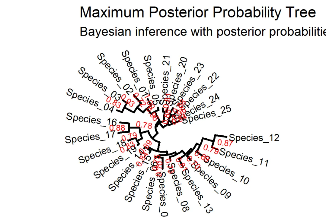
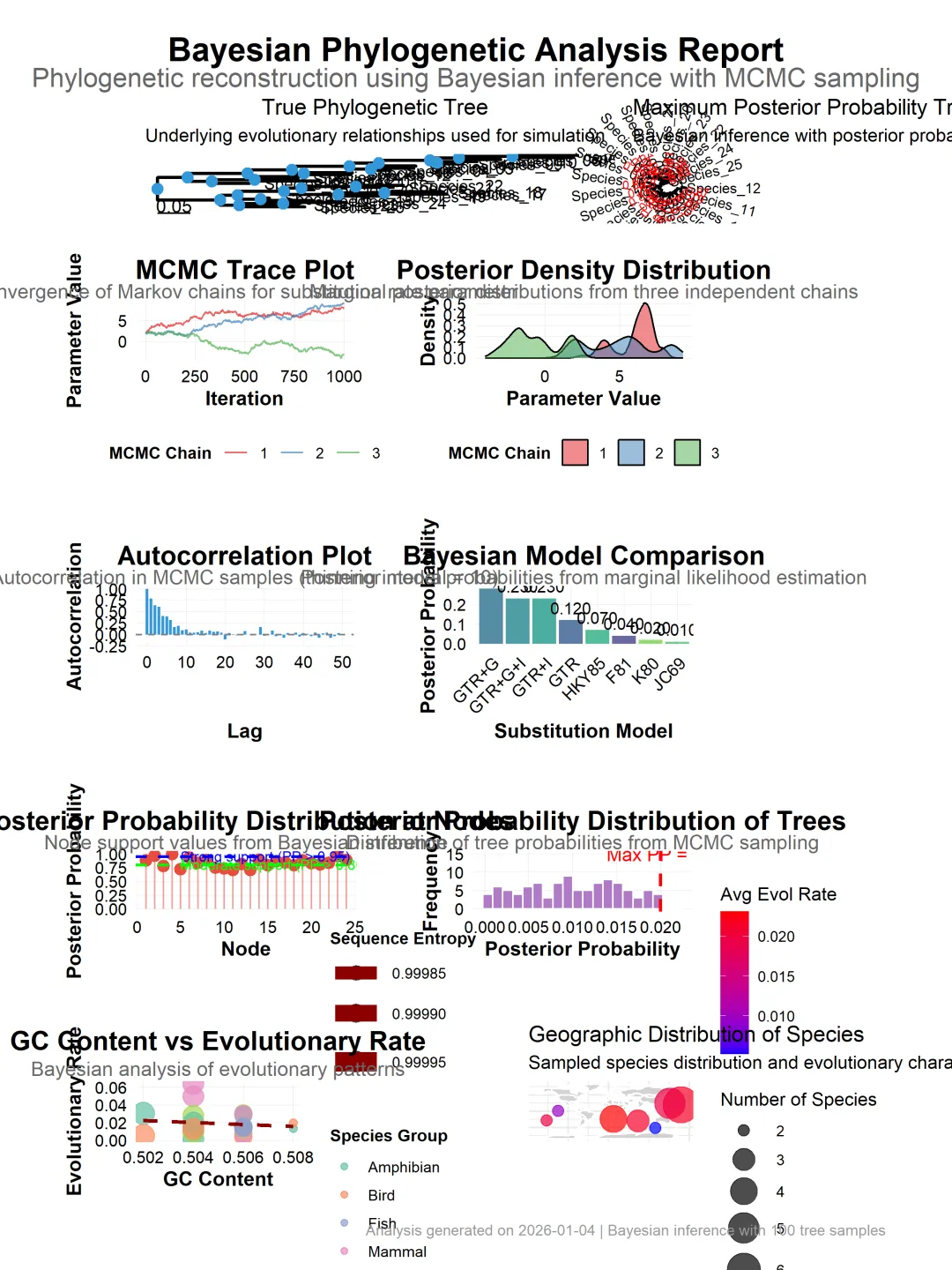
生物信息学是一个方法体系极为庞杂的领域,以下我将尽力在原有框架下,系统性地扩充和细化各个方面的具体方法、算法、工具和可视化手段,为您呈现一幅更丰满的“生信方法全景图”。
1.序列比对-基于Needleman-Wunsch动态规划算法的全局比对
2.序列比对-基于Smith-Waterman动态规划算法的局部比对
3.序列比对-采用BLAST等工具的启发式搜索
4.序列特征识别:基于隐马尔可夫模型(HMM)的序列特征识别
5.序列特征识别:基于权重矩阵的序列特征识别
6.比较基因组学:基于序列比对最大似然法的构建进化树系统发育重建
7.比较基因组学:基于序列比对贝叶斯推断的构建进化树系统发育重建
8.结构分析:同源建模:基于已知结构的同源蛋白预测目标蛋白结构
9.结构分析:分子对接:模拟小分子与蛋白质的相互作用(如AutoDock)
10.功能富集分析-超几何分布检验解读高通量实验筛选出的基因列表
11.功能富集分析-Fisher精确检验解读高通量实验筛选出的基因列表
12.功能富集分析-基因集富集分析解读高通量实验筛选出的基因列表
13.差异表达分析-基于计数模型的RNA-seq数据负二项分布模型统计检验
14.差异表达分析-基于线性模型的转录组数据的基因差异性识别
15.差异表达分析-基于经验贝叶斯模型的转录组数据的基因差异性识别
16.单细胞聚类与注释-使用PCA、t-SNE或UMAP等方法的降维
17.单细胞聚类与注释-Louvain、Leiden等图聚类算法
18.单细胞聚类与注释-通过查找比对已知的细胞类型标记基因定义生物学类型
19.蛋白质互作网络分析-基于基因融合、保守的基因邻接关系的基因组学方法进行网络构建
20.蛋白质互作网络分析-使用MCODE等算法识别紧密连接的功能模块的网络分析
21.系统发育分析-选择压力分析通过计算同义、非同义突变比率(dN/dS)的纯化选择、中性进化还是正选择判断
22.表观遗传学分析-对亚硫酸盐测序数据的DNA甲基化分析
23.表观遗传学分析-基于峰值检测的染色质可及性识别
24.表观遗传学分析-基于峰值检测的蛋白结合分析
25.空间转录组分析-基于SpatialDE、SPARK等统计模型空间变异基因识别
26.空间转录组分析-基于基因表达的空间相似性的空间域识别
27.空间转录组分析-跨多个组织切片的差异空间表达模式多切片比对与差异分析
28.多组学整合分析-关联分析:寻找不同组学层面数据间的统计相关性。
29.多组学整合分析-网络整合:构建包含多类型分子实体及它们之间多层次相互作用的整合网络。
30.多组学整合分析-基于多组学因子分析模型的因子分析与深度学习
31.机器学习与人工智能:监督学习:用已知标签训练分类器(如随机森林、深度学习)预测基因功能、蛋白结构
32.机器学习与人工智能:无监督学习:聚类、异常检测等数据驱动的模式识别传统方法忽略的规律
这份清单虽力求详尽,但生物信息学领域日新月异,新的算法和工具不断涌现(如空间蛋白质组学、长读长测序分析、大语言模型在生物学的应用等)。掌握这些方法的核心思想比记住所有工具名称更重要。在实际研究中,通常需要灵活组合多种方法,形成一条从原始数据到生物学发现的分析流水线。建议的学习路径是:先建立清晰的框架认知(如本回答),然后根据具体研究问题,深入钻研相关的一个或几个子领域。 希望这份扩展版的梳理能为您提供一张有价值的“导航地图”。
医学统计数据分析分享交流SPSS、R语言、Python、ArcGis、Geoda、GraphPad、数据分析图表制作等心得。承接数据分析,论文返修,医学统计,机器学习,生存分析,空间分析,问卷分析,生信分析业务。若有投稿和数据分析代做需求,可以直接联系我,谢谢!

“医学统计数据分析”公众号右下角;
找到“联系作者”,
可加我微信,邀请入粉丝群!

有临床流行病学数据分析
如(t检验、方差分析、χ2检验、logistic回归)、
(重复测量方差分析与配对T检验、ROC曲线)、
(非参数检验、生存分析、样本含量估计)、
(筛检试验:灵敏度、特异度、约登指数等计算)、
(绘制柱状图、散点图、小提琴图、列线图等)、
机器学习、深度学习、生存分析
等需求的同仁们,加入【临床】粉丝群。
疾控,公卫岗位的同仁,可以加一下【公卫】粉丝群,分享生态学研究、空间分析、时间序列、监测数据分析、时空面板技巧等工作科研自动化内容。
有实验室数据分析需求的同仁们,可以加入【生信】粉丝群,交流NCBI(基因序列)、UniProt(蛋白质)、KEGG(通路)、GEO(公共数据集)等公共数据库、基因组学转录组学蛋白组学代谢组学表型组学等数据分析和可视化内容。
或者可扫码直接加微信进群!!!




精品视频课程-“医学统计数据分析”视频号付费合集
在“医学统计数据分析”视频号-付费合集兑换相应课程后,获取课程理论课PPT、代码、基础数据等相关资料,请大家在【医学统计数据分析】公众号右下角,找到“联系作者”,加我微信后打包发送。感谢您的支持!!!
