期刊图片复现|Python绘制单特征shap依赖图+数据分布直方图组合图,含阈值计算及多项式拟合线
- 2026-10-11 06:15:26
期刊图片复现|Python绘制单特征shap依赖图+数据分布直方图组合图,含阈值计算及多项式拟合线

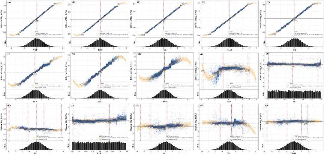
论文:Understanding the global subnational migration patterns driven by hydrological intrusion exposure 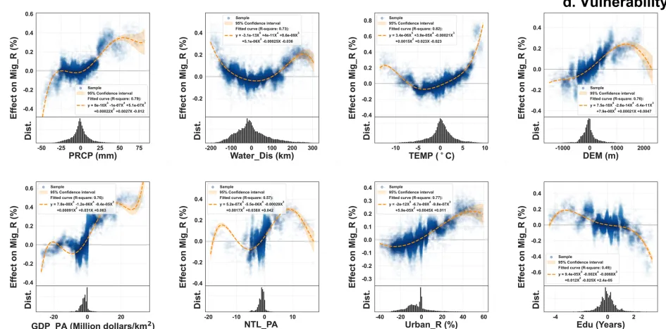
论文原图 这张shap依赖图揭示了特征ASP的变化对目标FVC的影响。上半部分揭示了ASP特征与其对预测的影响之间存在一个复杂的非线性关系:当ASP值低于-0.83时,它对FVC为负面影响;高于-0.83时,转变为了正向的影响;而当ASP值超过2.42后,其影响再次转为负面并急剧下降。橙色虚线为五次多项式拟合曲线,阴影区域为了95%的置信区间。 图的下半部分是一个直方图,展示了ASP特征本身的数据分布情况,可以看出其数值主要集中在-2到2的范围内,呈近似正态的分布。 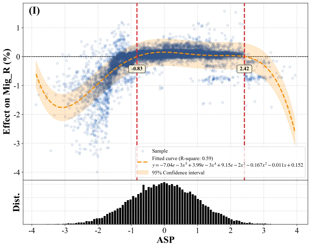
仿图 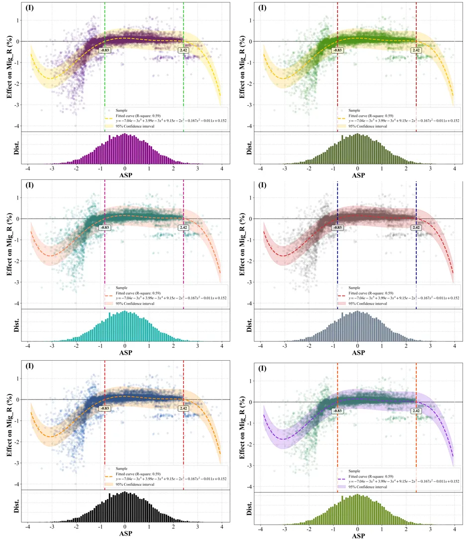




导入库与全局样式配置,是代码实现的基础同时也是绘图前的准备工作。 

颜色库设置 

单特征依赖图绘图函数,这部分要记得修改结果的输出位置 

这个还是用的那一套代码,看过之前文章的人应该有印象,就是生成子图后粘贴到一个新的大图上 

数据的加载与处理 读取原始数据,提取特征数据和目标变量,划分训练集和测试集、标准化处理等 主要修改的位置都集中在这里 

模型构建,超参数是我瞎弄得,一定要记得修改啊 

模型的性能评估及最佳模型保存 

模SHAP分析 

绘图 



期刊图片复现|Python绘制二维偏依赖PDP图 期刊复现|python绘制基于SHAP分析和GAM模型拟合的单特征依赖图 期刊图片复现|python绘制带有渐变颜色shap特征重要性组合图(条形图+蜂巢图) 期刊复现|用Python绘制SHAP特征重要性总览图、依赖图、双特征交互效应SHAP图,解锁XGBoost模型的终极奥秘 期刊图片复现|Python绘制shap重要性蜂巢图+单特征依赖图+交互效应强度气泡图+交互效应依赖图(回归+二分类+分类) 



需要的请后台私信我获取详细信息,注意只会分享练习数据和代码文件,不会提供答疑服务,代码文件中已经包含了每行代码的完整注释!!!
代码绘制成果展示
代码解释
第一部分
# =========================================================================================# ======================================1.库的导入=========================================# =========================================================================================import numpy as npimport matplotlib.pyplot as pltimport lightgbm as lgbimport shapimport pandas as pdimport joblibfrom sklearn.model_selection import train_test_split, GridSearchCVfrom sklearn.preprocessing import StandardScalerfrom sklearn.metrics import r2_score, mean_squared_errorimport osfrom PIL import Imageplt.rcParams['font.family'] = 'serif'plt.rcParams['font.serif'] = ['Times New Roman']plt.rcParams['axes.unicode_minus'] = Falseplt.rcParams['mathtext.fontset'] = 'stix'import matplotlibmatplotlib.rcParams['pdf.fonttype'] = 42matplotlib.rcParams['ps.fonttype'] = 42
第二部分
# =========================================================================================# ======================================2.颜色库设置=========================================# =========================================================================================color_schemes = {1: {'scatter': '#0047AB', 'fit': 'darkorange', 'fill': 'darkorange','threshold_line': '#E3242B', 'threshold_text_bg': '#FFF8DC', 'histogram': 'black'},}selected_scheme = 7#选择配色colors = color_schemes.get(selected_scheme, color_schemes[1])
第三部分
# =========================================================================================# ======================================3.单特征依赖图绘图函数================================# =========================================================================================def plot_shap_dependence(feature_name, feature_values, shap_values_for_feature, plot_index, colors,save_dir='output_plots'):print(f"正在处理:{feature_name}")fig = plt.figure(figsize=(10, 8))gs = fig.add_gridspec(2, 1, height_ratios=[4, 1], hspace=0)ax1 = fig.add_subplot(gs[0, 0])ax2 = fig.add_subplot(gs[1, 0], sharex=ax1)plt.tight_layout()#保存os.makedirs(save_dir, exist_ok=True)file_path_png = os.path.join(save_dir,fr'shap_dependence_{feature_name}_{selected_scheme}.png')file_path_pdf = os.path.join(save_dir,fr'shap_dependence_{feature_name}_{selected_scheme}.pdf')plt.savefig(file_path_png, dpi=300, bbox_inches='tight')plt.savefig(file_path_pdf, bbox_inches='tight')plt.close(fig)return file_path_png
第四部分
# =========================================================================================# ======================================4.拼接函数=========================================# =========================================================================================def stitch_images_grid(image_paths, n_cols, output_filename_base, save_dir):images = [Image.open(path) for path in image_paths]img_width, img_height = images[0].sizen_images = len(images)n_rows = (n_images + n_cols - 1) // n_colstotal_width = n_cols * img_widthtotal_height = n_rows * img_heightcomposite_image = Image.new('RGB', (total_width, total_height), color='white')for i, img in enumerate(images):row = i // n_colscol = i % n_colspaste_x = col * img_widthpaste_y = row * img_heightcomposite_image.paste(img, (paste_x, paste_y))img.close()png_path_composite = os.path.join(save_dir, f"{output_filename_base}.png")composite_image.save(png_path_composite)print(f"\n组合图已保存为 '{png_path_composite}'")pdf_path_composite = os.path.join(save_dir, f"{output_filename_base}.pdf")if composite_image.mode == 'RGBA':composite_image = composite_image.convert('RGB')composite_image.save(pdf_path_composite)print(f"组合图已保存为 '{pdf_path_composite}'")
第五部分
# =========================================================================================# ======================================5.数据的加载与处理=========================================# =========================================================================================file_path = r'data.xlsx'target_column_name = 'FVC'data_df = pd.read_excel(file_path)print(f"成功从 '{file_path}' 加载数据。")feature_names = [col for col in data_df.columns if col != target_column_name]X = data_df[feature_names]y = data_df[target_column_name]print(f"特征列表: {feature_names}")X_train, X_test, y_train, y_test = train_test_split(X, y, test_size=0.2, random_state=42)scaler = StandardScaler()X_train_scaled = scaler.fit_transform(X_train)X_test_scaled = scaler.transform(X_test)X_train_scaled = pd.DataFrame(X_train_scaled, columns=X_train.columns, index=X_train.index)X_test_scaled = pd.DataFrame(X_test_scaled, columns=X_test.columns, index=X_test.index)
第六部分
# =========================================================================================# ======================================6.模型构建=========================================# =========================================================================================print("\n--- 正在使用GridSearchCV训练LGBM模型 ---")lgb_model = lgb.LGBMRegressor(random_state=42)param_grid = {'n_estimators': [100, 200, 300],# 'max_depth': [3, 5, 7],# 'learning_rate': [0.01, 0.05, 0.1],# 'num_leaves': [20, 31, 40]}grid_search = GridSearchCV(estimator=lgb_model,param_grid=param_grid,cv=3,n_jobs=-1,scoring='neg_mean_squared_error',verbose=1)grid_search.fit(X_train_scaled, y_train)print(f"最佳超参数: {grid_search.best_params_}")best_model = grid_search.best_estimator_
第七部分
# =========================================================================================# ======================================7.模型性能评估=========================================# =========================================================================================print("\n模型性能")y_train_pred = best_model.predict(X_train_scaled)r2_train = r2_score(y_train, y_train_pred)mse_train = mean_squared_error(y_train, y_train_pred)print(f"训练集:R2: {r2_train:.4f} | MSE: {mse_train:.4f}")y_test_pred = best_model.predict(X_test_scaled)r2_test = r2_score(y_test, y_test_pred)mse_test = mean_squared_error(y_test, y_test_pred)print(f"测试集:R2: {r2_test:.4f} | MSE: {mse_test:.4f}")output_dir = r"saved_model_and_data"model_path = os.path.join(output_dir, 'best_lgbm_model.joblib')joblib.dump(best_model, model_path)
第八部分
# =========================================================================================# ======================================8.shap分析=========================================# =========================================================================================print("\n计算SHAP值")explainer = shap.TreeExplainer(best_model)shap_values_matrix = explainer.shap_values(X_test_scaled)feature_importance = np.abs(shap_values_matrix).mean(axis=0)sorted_feature_indices = np.argsort(feature_importance)[::-1]feature_name_to_original_index = {name: i for i, name in enumerate(feature_names)}sorted_feature_names = [feature_names[i] for i in sorted_feature_indices]print(f"特征按重要性排序: {sorted_feature_names}")
第九部分
# =========================================================================================# ======================================9.绘图,包括子图和组合图=========================================# =========================================================================================saved_plot_paths = []for plot_idx, sorted_name in enumerate(sorted_feature_names):original_idx = feature_name_to_original_index[sorted_name]plot_path = plot_shap_dependence(feature_name=sorted_name,feature_values=X_test.iloc[:, original_idx],shap_values_for_feature=shap_values_matrix[:, original_idx],plot_index=plot_idx,colors=colors,save_dir='output_shap_plots')saved_plot_paths.append(plot_path)n_cols_for_stitching = 5output_filename_base = f"composite_{selected_scheme}"output_save_dir = r'shap依赖图+多项式拟合+直方图'stitch_images_grid(image_paths=saved_plot_paths,n_cols=n_cols_for_stitching,output_filename_base=output_filename_base,save_dir=output_save_dir)
如何应用?
1.选择配色方案:
selected_scheme = 7#选择配色2.设置子图的保存地址:
file_path_png = os.path.join(save_dir,fr'shap依赖图+多项式拟合+直方图\shap_dependence_{feature_name}_{selected_scheme}.png')file_path_pdf = os.path.join(save_dir,fr'shap依赖图+多项式拟合+直方图\shap_dependence_{feature_name}_{selected_scheme}.pdf')
3.设置数据的输入地址:
file_path = r'\data.xlsx' # 指定Excel文件的路径4.定义目标变量:
target_column_name = 'FVC' #目标变量5.设置数据集的划分:
X_train, X_test, y_train, y_test = train_test_split(X, y, test_size=0.2, random_state=42)6.设置超参数:
param_grid = {'n_estimators': [100, 200, 300],# 'max_depth': [3, 5, 7],# 'learning_rate': [0.01, 0.05, 0.1],# 'num_leaves': [20, 31, 40] }
7.最佳模型的保存路径:
output_dir = r"saved_model_and_data"8.设置组合图的文件名和保存地址:
output_filename_base = f"composite_{selected_scheme}" #组合图的文件名output_save_dir = r'shap依赖图+多项式拟合+直方图' #组合图的保存地址
推荐
预告
获取方式
本文来自网友投稿或网络内容,如有侵犯您的权益请联系我们删除,联系邮箱:596563534@qq.com 。
随机文章
-
 10个月宝宝每天需要喝多少奶粉?
- 怎么看懂Python代码,看一遍就会
- HiMCM建模工具箱怎么配?Python与MATLAB实战对比,附2026备考资源
- 这5个Python库一旦掌握就离不开
- 用Python 画出高颜值柱状图 | 数据分析直接封神
- python实现北半球投影绘图-适用于离散型 数据
- 10个常用的python人工智能AI库
- 【python3.7.3setup】python3.7.3setup完整安装激活步骤及python安装包下载
- 实用Python代码1:宽格式表转长格式表
- Python 处理JSON/接口高性能序列化神器:orjson
- Python之实现文本转语音-edge-tts