从BS公式到蒙特卡洛:6张Python图拆解0DTE末日轮

0DTE是Zero Days to Expiration的缩写，指的是当天到期的期权合约。这类合约在美股市场极为活跃，尤其是SPX、SPY等指数的周一、周三、周五到期合约。0DTE策略的核心吸引力在于它把期权交易中最极端的两个特征Gamma的爆炸式增长和Theta的加速衰减压缩到了短短几个小时之内。理解这两个力量的相互作用，是掌握0DTE交易的钥匙。老规矩所有代码放在文末，欢迎自取。一、Gamma尖峰：0DTE的物理本质在Black-Scholes框架下，期权的Gamma衡量的是Delta对标的价格的敏感度。对于平值（ATM）期权，Gamma有一个简洁的近似表达式：Gamma与剩余期限的平方根成反比。这意味着当到期日临近时，Gamma会以τ^(-1/2)的速度发散。一个一年期的ATM期权，Gamma可能只有0.02；而当期限压缩到一天，Gamma会膨胀到0.3以上；在最后一个小时，Gamma可以达到0.8以上，是一年期期权的四十余倍；若是进入最后几分钟，Gamma突破4也并非难事。这种爆炸不是线性的，而是指数级的，每过一分钟，期权对价格变动的敏感度都在以更快的速度增长。下图展示了这个过程的完整图景。左上角的子图绘制了不同剩余期限下Gamma随标的价格的分布曲线。当τ=1年时，Gamma在ATM附近呈现一个平缓的钟形；随着期限缩短到0.25年、0.05年，钟形逐渐变窄变高；当τ=0.001年（约0.25天）时，曲线在K=100处收缩成一个极其尖锐的单峰，峰宽极窄，两侧迅速跌落至零。这意味着在0DTE场景下，一旦标的价格偏离执行价哪怕一点点，Gamma就会迅速坍缩，期权的弹性瞬间消失。右上角的Theta分布呈现对称的深谷形态，ATM处的Theta绝对值最大，时间价值蒸发最快。

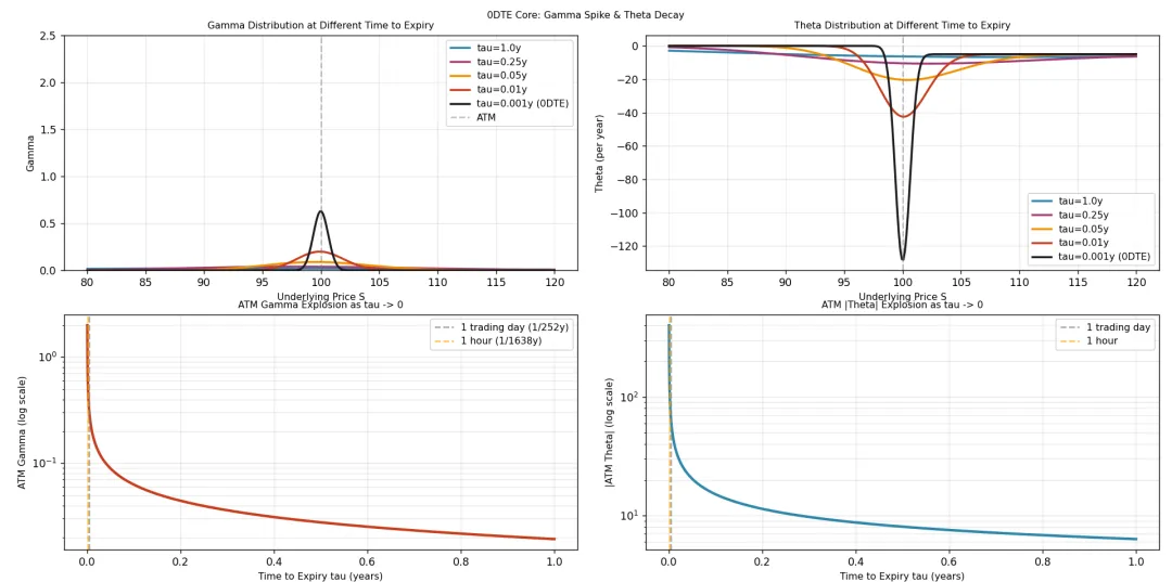
下方的两个对数坐标图更直观地揭示了极限行为。左下图显示ATM Gamma随剩余期限的变化：在1个交易日（1/252年）处，Gamma已经显著抬升；而在1小时（1/1638年）处，曲线垂直上冲，数值达到一年期期权的数十倍以上。右下图的|Theta|呈现完全相同的形态。这两张图合在一起，构成了0DTE策略的底层物理图景：你面对的是一个Gamma和Theta同时趋于无穷大的奇异点，任何微小的价格扰动都会被极度放大，而时间价值的流失速度也在以指数级加速。二、跨式组合的盈亏结构在0DTE策略中，最经典的结构是跨式组合（Straddle），即同时买入或卖出同一执行价的认购和认沽期权。这种结构完全对称，不赌方向，只赌波动。Long Straddle的盈利逻辑是：支付一笔权利金，换取标的价格向任意方向大幅波动的收益；Short Straddle则相反，收取权利金，承担价格大幅波动的风险。下图左侧展示了Long Straddle在一天到期时的盈亏曲线。蓝色实线是期权当前价格，红色虚线是到期 payoff，黑色实线是扣除成本后的P&L。由于时间价值尚未完全蒸发，当前价格曲线在ATM处形成一个圆润的底部，略高于到期 payoff 的尖底。绿色区域代表盈利区，红色区域代表亏损区。可以看到，盈亏平衡点位于执行价两侧约1个单位处。这意味着标的价格当天需要波动超过1%才能覆盖权利金成本。

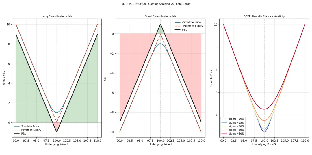
中间的Short Straddle呈现完全镜像的倒V型。卖方在ATM附近获得最大收益，但一旦价格突破盈亏平衡点，亏损斜率为1，理论上无上限。右侧子图展示了不同波动率假设下的Straddle价格。波动率越高，Straddle越贵，底部越宽。在0DTE场景下，这个底部宽度直接决定了策略的容错空间：高IV环境下买入Straddle成本高昂，需要更大的价格波动才能盈利；而卖出Straddle则因为收取了更多保费，获得了更厚的安全垫。三、蒙特卡洛模拟：用路径说话希腊字母给出了瞬时的敏感度，但无法告诉你策略在真实市场环境下的期望表现。蒙特卡洛模拟的价值在于，它通过生成成千上万条符合几何布朗运动的价格路径，让你直观地看到策略盈亏的概率分布。这里我们完全沿用前文提供的向量化代码风格：利用numpy的cumsum在矩阵维度上批量生成路径，运算效率远高于逐路径循环。

我们设定标的初始价格100，执行价100，年化波动率20%，无风险利率5%，股息率2%，模拟5000条路径，每条路径50个时间步，覆盖一个完整的交易日。下图左上方展示了其中20条代表性路径，可以看到在6.5小时的交易时间内，价格大致在98到102之间波动，符合20%年化波动率下一天内的理论波动范围。右上方是到期价格的直方图，呈现标准的对数正态分布，均值约100.01，与理论预期一致。

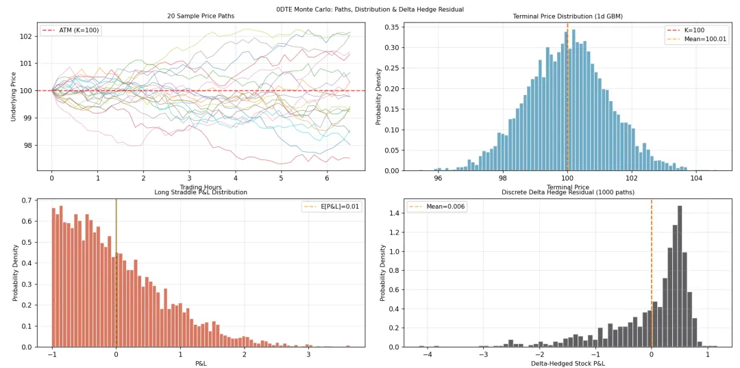
左下方的Long Straddle P&L分布揭示了一个关键事实：在Black-Scholes假设下，期望P&L趋近于零，但分布严重右偏。大量路径集中在-1附近（亏损全部权利金），少数路径向右延伸，形成长尾。这意味着Long Straddle是一个小概率大赚、大概率小亏的策略，其正期望值完全依赖于实际波动率高于隐含波动率。右下方展示了离散Delta对冲后的残余风险分布。在理论上，如果对冲是连续且完美的，股票对冲头寸的盈亏应与期权持仓的Gamma收益精确抵消；但在离散时间、高Gamma的0DTE环境中，再平衡间隔内价格的跳跃会导致残余风险。模拟结果显示这一残余分布以零为中心，均值0.006，说明离散化误差在统计上可控，但尾部仍然存在不可忽视的敞口。四、日内动态：最后一小时的决战0DTE策略最惊心动魄的阶段是到期前的最后一两个小时。下图通过一条随机生成的价格路径，展示了Gamma、Theta和Delta在日内如何演化。

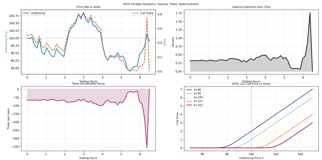
左上图双轴展示了标的价格与Call Delta的联动关系。可以清晰看到，在交易前5小时，Delta在0.4到0.6之间温和波动；但在最后30分钟，当价格跌破99时，Delta从0.3断崖式下跌至接近0，这种跳跃的幅度和速度在常规期限期权中极为罕见。右上图的Gamma曲线更为震撼。在前5个小时，Gamma维持在0.3到0.5的相对平稳区间；进入最后1小时，Gamma开始急剧拉升，在临近到期时突破1.5，形成垂直上冲。这意味着同样的价格变动，在最后10分钟造成的Delta调整是开盘时的3到5倍。左下图的Theta曲线同步呈现加速下探，最后阶段的Theta绝对值达到-350以上（年化），时间价值以分钟为单位在蒸发。右下图展示了距离到期1小时时，不同执行价的Call价格曲线。K=98的深实值Call几乎与标的价格同步线性上涨；K=102的虚值Call则在ATM右侧缓慢抬升；而K=100的平值Call在ATM处呈现最尖锐的转折。这组曲线直观地说明，在0DTE的最后阶段，平值期权的价格行为最接近二元彩票，它要么迅速变成实值，要么迅速归零，中间过渡带极窄。五、策略对比与风险分布跨式组合并非0DTE的唯一选择。宽跨式（Strangle）通过买入不同执行价的Call和Put，降低了权利金成本，但牺牲了ATM附近的盈利空间。下图左上方对比了三种策略的到期盈亏：Long Straddle（蓝）在ATM处亏损最大，但两侧盈利斜率陡峭；Long Strangle（紫，执行价98/102）在98到102之间完全亏损，但成本更低；Short Straddle（红）呈现倒V型，收取保费但承担尾部风险。

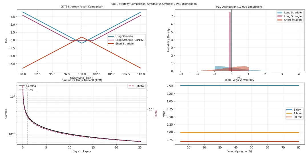
右上方通过10000次蒙特卡洛模拟展示了三种策略的P&L概率分布。Short Straddle的分布极度左偏，峰值集中在0附近，左侧有长尾，这对应着大概率赚小钱，小概率亏大钱的特征。Long Straddle和Strangle则呈现右偏，多数路径亏损，少数路径获得高额回报。左下方的对数坐标图揭示了Gamma与Theta的权衡关系：两者随剩余期限同步爆炸，你无法只取其一。右下方的Vega分析则表明，0DTE的Vega极低且对波动率水平不敏感，这意味着0DTE本质上是方向性/波动率博弈，而非Vega交易。六、隐含波动率的定价博弈0DTE策略的盈亏归根结底取决于一个核心问题：市场定价的隐含波动率（IV）是否准确反映了实际将要发生的波动？下图展示了一个思想实验：假设实际波动率固定为20%，我们按照不同的IV水平卖出Straddle，然后观察期望P&L。

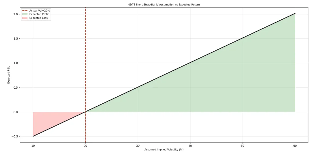
横轴是假设的IV水平，纵轴是期望盈亏。当IV=20%时，直线穿过零点，公平博弈，长期期望为零。当IV高于20%，卖方获得正期望收益，且收益与IV溢价呈线性关系；当IV低于20%，卖方亏损。绿色区域代表预期盈利区，红色区域代表预期亏损区。这张图揭示了0DTE交易的核心逻辑：你不是在交易方向，而是在交易市场对当天波动率的预期误差。在FOMC、CPI发布、财报公布等事件日，IV往往被过度定价，此时卖出Straddle的期望收益为正；而在平静交易日，IV可能被低估，买方占据优势。

import mathimport numpy as npimport matplotlib.pyplot as pltfrom scipy.integrate import quaddef dN(x):return math.exp(-0.5 * x**2) / math.sqrt(2 * math.pi)def N(d):return quad(lambda x: dN(x), -20, d, limit=50)[0]def d1f(S, K, t, T, r, q, sigma):    tau = T - tif tau <= 0:        tau = 1e-6d1 = (math.log(S / K) + (            r - q + 0.5 * sigma**2) * tau) / (sigma * math.sqrt(tau))return d1def call_value(S, K, t, T, r, q, sigma):    tau = max(T - t, 1e-6)    d1 = d1f(S, K, t, T, r, q, sigma)    d2 = d1 - sigma * math.sqrt(tau)return N(d1) * S * math.exp(-q * tau) - N(d2) * K * math.exp(-r * tau)def put_value(S, K, t, T, r, q, sigma):    tau = max(T - t, 1e-6)    d1 = d1f(S, K, t, T, r, q, sigma)    d2 = d1 - sigma * math.sqrt(tau)return -S * N(-d1) * math.exp(-q * tau) + math.exp(-r * tau) * K * N(-d2)def delta(S, K, t, T, r, q, sigma):return N(d1f(S, K, t, T, r, q, sigma))def gamma(S, K, t, T, r, q, sigma):    tau = max(T - t, 1e-6)    d1 = d1f(S, K, t, T, r, q, sigma)return dN(d1) / (S * sigma * math.sqrt(tau))def theta(S, K, t, T, r, q, sigma):    tau = max(T - t, 1e-6)    d1 = d1f(S, K, t, T, r, q, sigma)    d2 = d1 - sigma * math.sqrt(tau)return -((S * dN(d1) * sigma) / (2 * math.sqrt(tau))) - r * K * math.exp(-r * tau) * N(d2)def vega(S, K, t, T, r, q, sigma):    tau = max(T - t, 1e-6)    d1 = d1f(S, K, t, T, r, q, sigma)return S * dN(d1) * math.sqrt(tau)def mc_call_value(S0, K, r, q, T, sigma, M, I):    dt = T / M    S = S0 * np.exp(np.cumsum(        (r - q - 0.5 * sigma**2) * dt + sigma *        np.sqrt(dt) * np.random.standard_normal((M + 1, I)), axis=0))    S[0] = S0    optionvalue = np.exp(-r * T) * np.sum(np.maximum(S[-1] - K, 0)) / Ireturn optionvalue, Sdef mc_put_value(S0, K, r, q, T, sigma, M, I):    dt = T / M    S = S0 * np.exp(np.cumsum(        (r - q - 0.5 * sigma**2) * dt + sigma *        np.sqrt(dt) * np.random.standard_normal((M + 1, I)), axis=0))    S[0] = S0    optionvalue = np.exp(-r * T) * np.sum(np.maximum(K - S[-1], 0)) / Ireturn optionvalue, SK = 100r = 0.05q = 0.02sigma = 0.20T = 1.0S0 = 100tau = 1 / 252       # 1 trading dayS_range = np.linspace(80, 120, 300)# Figure 1: Gamma Spike & Theta Decayfig, axes = plt.subplots(2, 2, figsize=(14, 10))fig.suptitle('0DTE Core: Gamma Spike & Theta Decay', fontsize=9, y=0.98)ax1 = axes[0, 0]tau_vals = [1.0, 0.25, 0.05, 0.01, 0.001]colors = ['#2E86AB', '#A23B72', '#F18F01', '#C73E1D', '#1B1B1E']labels = ['tau=1.0y', 'tau=0.25y', 'tau=0.05y','tau=0.01y', 'tau=0.001y (0DTE)']for tau_v, color, label in zip(tau_vals, colors, labels):    t = T - tau_v    g = [gamma(S, K, t, T, r, q, sigma) for S in S_range]    ax1.plot(S_range, g, color=color, linewidth=2, label=label)ax1.axvline(x=K, color='gray', linestyle='--', alpha=0.5, label='ATM')ax1.set_xlabel('Underlying Price S', fontsize=9)ax1.set_ylabel('Gamma', fontsize=9)ax1.set_title('Gamma Distribution at Different Time to Expiry', fontsize=9)ax1.legend(loc='upper right', fontsize=9)ax1.set_ylim(0, 2.5)ax1.grid(True, alpha=0.3)ax2 = axes[0, 1]for tau_v, color, label in zip(tau_vals, colors, labels):    t = T - tau_v    th = [theta(S, K, t, T, r, q, sigma) for S in S_range]    ax2.plot(S_range, th, color=color, linewidth=2, label=label)ax2.axvline(x=K, color='gray', linestyle='--', alpha=0.5)ax2.set_xlabel('Underlying Price S', fontsize=9)ax2.set_ylabel('Theta (per year)', fontsize=9)ax2.set_title('Theta Distribution at Different Time to Expiry', fontsize=9)ax2.legend(loc='lower right', fontsize=9)ax2.grid(True, alpha=0.3)ax3 = axes[1, 0]tau_fine = np.logspace(-4, 0, 200)atm_g = [gamma(K, K, 1.0 - t, 1.0, r, q, sigma) for t in tau_fine]ax3.semilogy(tau_fine, atm_g, color='#C73E1D', linewidth=2.5)ax3.axvline(x=1/252, color='gray', linestyle='--',alpha=0.7, label='1 trading day (1/252y)')ax3.axvline(x=1/(252*6.5), color='orange', linestyle='--',alpha=0.7, label='1 hour (1/1638y)')ax3.set_xlabel('Time to Expiry tau (years)', fontsize=9)ax3.set_ylabel('ATM Gamma (log scale)', fontsize=9)ax3.set_title('ATM Gamma Explosion as tau -> 0', fontsize=9)ax3.legend(loc='upper right', fontsize=9)ax3.grid(True, alpha=0.3, which='both')ax4 = axes[1, 1]atm_th = [abs(    theta(K, K, 1.0 - t, 1.0, r, q,sigma)) for t in tau_fine]ax4.semilogy(tau_fine, atm_th, color='#2E86AB', linewidth=2.5)ax4.axvline(x=1/252, color='gray', linestyle='--',alpha=0.7, label='1 trading day')ax4.axvline(x=1/(252*6.5), color='orange', linestyle='--',alpha=0.7, label='1 hour')ax4.set_xlabel('Time to Expiry tau (years)', fontsize=9)ax4.set_ylabel('|ATM Theta| (log scale)', fontsize=9)ax4.set_title('ATM |Theta| Explosion as tau -> 0', fontsize=9)ax4.legend(loc='upper right', fontsize=9)ax4.grid(True, alpha=0.3, which='both')plt.tight_layout()plt.savefig('fig1_gamma_theta.png', dpi=150, bbox_inches='tight')plt.show()# Figure 2: Straddle P&L Profilefig, axes = plt.subplots(1, 3, figsize=(16, 5))fig.suptitle('0DTE P&L Structure: '             'Gamma Scalping vs Theta Decay', fontsize=9, y=0.98)S_range2 = np.linspace(90, 110, 300)ax1 = axes[0]call_p = [call_value(S, K, 0, tau, r, q, sigma) for S in S_range2]put_p = [put_value(S, K, 0, tau, r, q, sigma) for S in S_range2]straddle_p = [c + p for c, p in zip(call_p, put_p)]cost = call_value(K, K, 0, tau, r, q, sigma)\       + put_value(K, K, 0, tau, r, q, sigma)payoff = [max(S - K, 0) + max(K - S, 0) for S in S_range2]pl = [p - cost for p in payoff]ax1.plot(S_range2, straddle_p, color='#2E86AB',linewidth=2, label='Straddle Price')ax1.plot(S_range2, payoff, color='#C73E1D',linewidth=2, linestyle='--', label='Payoff at Expiry')ax1.plot(S_range2, pl, color='#1B1B1E', linewidth=2.5, label='P&L')ax1.axhline(y=0, color='gray', linestyle='-', alpha=0.3)ax1.axvline(x=K, color='gray', linestyle='--', alpha=0.3)ax1.fill_between(S_range2, pl, 0,where=[p >= 0 for p in pl], alpha=0.2, color='green')ax1.fill_between(S_range2, pl, 0,where=[p < 0 for p in pl], alpha=0.2, color='red')ax1.set_xlabel('Underlying Price S', fontsize=9)ax1.set_ylabel('Value / P&L', fontsize=9)ax1.set_title('Long Straddle (tau=1d)', fontsize=9)ax1.legend(fontsize=9)ax1.grid(True, alpha=0.3)ax2 = axes[1]pl_short = [-p for p in pl]ax2.plot(S_range2, [-s for s in straddle_p],color='#2E86AB', linewidth=2, label='-Straddle Price')ax2.plot(S_range2, [-p for p in payoff],color='#C73E1D', linewidth=2, linestyle='--', label='-Payoff at Expiry')ax2.plot(S_range2, pl_short, color='#1B1B1E', linewidth=2.5, label='P&L')ax2.axhline(y=0, color='gray', linestyle='-', alpha=0.3)ax2.axvline(x=K, color='gray', linestyle='--', alpha=0.3)ax2.fill_between(S_range2, pl_short, 0,where=[p >= 0 for p in pl_short], alpha=0.2, color='green')ax2.fill_between(S_range2, pl_short, 0,where=[p < 0 for p in pl_short], alpha=0.2, color='red')ax2.set_xlabel('Underlying Price S', fontsize=9)ax2.set_ylabel('P&L', fontsize=9)ax2.set_title('Short Straddle (tau=1d)', fontsize=9)ax2.legend(fontsize=9)ax2.grid(True, alpha=0.3)ax3 = axes[2]sigma_vals = [0.10, 0.15, 0.20, 0.30, 0.50]colors2 = plt.cm.RdYlBu_r(np.linspace(0, 1, len(sigma_vals)))for sig, color in zip(sigma_vals, colors2):    prices = [call_value(S, K, 0, tau, r, q, sig) +              put_value(S, K, 0, tau, r, q, sig) for S in S_range2]    ax3.plot(S_range2, prices,color=color, linewidth=2, label=f'sigma={sig*100:.0f}%')ax3.axvline(x=K, color='gray', linestyle='--', alpha=0.3)ax3.set_xlabel('Underlying Price S', fontsize=9)ax3.set_ylabel('Straddle Price', fontsize=9)ax3.set_title('0DTE Straddle Price vs Volatility', fontsize=9)ax3.legend(fontsize=9)ax3.grid(True, alpha=0.3)plt.tight_layout()plt.savefig('fig2_straddle_pl.png', dpi=150, bbox_inches='tight')plt.show()# Figure 3: Monte Carlo Simulationnp.random.seed(42)M_mc = 50I_mc = 5000dt_mc = tau / M_mcS_mc = S0 * np.exp(np.cumsum(    (r - q - 0.5 * sigma**2) * dt_mc + sigma *    np.sqrt(dt_mc) * np.random.standard_normal((M_mc + 1, I_mc)), axis=0))S_mc[0] = S0times_mc = np.linspace(0, tau, M_mc + 1)hours_mc = times_mc * 252 * 6.5fig, axes = plt.subplots(2, 2, figsize=(14, 10))fig.suptitle('0DTE Monte Carlo: Paths, Distribution '    '& Delta Hedge Residual', fontsize=9, y=0.98)ax1 = axes[0, 0]for i in range(20):    ax1.plot(hours_mc, S_mc[:, i], alpha=0.6, linewidth=0.8)ax1.axhline(y=K, color='red', linestyle='--', alpha=0.7, label='ATM (K=100)')ax1.set_xlabel('Trading Hours', fontsize=9)ax1.set_ylabel('Underlying Price', fontsize=9)ax1.set_title('20 Sample Price Paths', fontsize=9)ax1.legend(fontsize=9)ax1.grid(True, alpha=0.3)ax2 = axes[0, 1]ax2.hist(S_mc[-1], bins=80,color='#2E86AB', alpha=0.7, edgecolor='white', density=True)ax2.axvline(x=K, color='red', linestyle='--', alpha=0.7, label='K=100')ax2.axvline(x=np.mean(S_mc[-1]),color='orange', linestyle='--', alpha=0.7,label=f'Mean={np.mean(S_mc[-1]):.2f}')ax2.set_xlabel('Terminal Price', fontsize=9)ax2.set_ylabel('Probability Density', fontsize=9)ax2.set_title('Terminal Price Distribution (1d GBM)', fontsize=9)ax2.legend(fontsize=9)ax2.grid(True, alpha=0.3)ax3 = axes[1, 0]cost_mc = call_value(S0, K, 0, tau, r, q, sigma) + \          put_value(S0, K, 0, tau, r, q, sigma)straddle_pl_mc = np.maximum(S_mc[-1] - K, 0) + \                 np.maximum(K - S_mc[-1], 0) - cost_mcax3.hist(straddle_pl_mc, bins=80,color='#C73E1D', alpha=0.7, edgecolor='white', density=True)ax3.axvline(x=0, color='black', linestyle='-', alpha=0.5)ax3.axvline(x=np.mean(straddle_pl_mc), color='orange', linestyle='--',alpha=0.7, label=f'E[P&L]={np.mean(straddle_pl_mc):.2f}')ax3.set_xlabel('P&L', fontsize=9)ax3.set_ylabel('Probability Density', fontsize=9)ax3.set_title('Long Straddle P&L Distribution', fontsize=9)ax3.legend(fontsize=9)ax3.grid(True, alpha=0.3)ax4 = axes[1, 1]residual_pl = []for i in range(min(1000, I_mc)):    pl = 0.0position = 0.0for step in range(M_mc):        St = S_mc[step, i]        elapsed = step * dt_mc# Pass elapsed time as t, total tau as T for correct semanticd = delta(St, K, elapsed, tau, r, q, sigma)        new_pos = -d        pl += position * (S_mc[step + 1, i] - St)        position = new_pos    residual_pl.append(pl)residual_pl = np.array(residual_pl)ax4.hist(residual_pl, bins=60, color='#1B1B1E',alpha=0.7, edgecolor='white', density=True)ax4.axvline(x=0, color='red', linestyle='--', alpha=0.7)ax4.axvline(x=np.mean(residual_pl), color='orange', linestyle='--',alpha=0.7, label=f'Mean={np.mean(residual_pl):.3f}')ax4.set_xlabel('Delta-Hedged Stock P&L', fontsize=9)ax4.set_ylabel('Probability Density', fontsize=9)ax4.set_title('Discrete Delta Hedge Residual (1000 paths)', fontsize=9)ax4.legend(fontsize=9)ax4.grid(True, alpha=0.3)plt.tight_layout()plt.savefig('fig3_monte_carlo.png', dpi=150, bbox_inches='tight')plt.show()# Figure 4: Intraday Dynamicsnp.random.seed(123)M_id = 50dt_id = tau / M_idS_id = S0 * np.exp(    np.cumsum((r - q - 0.5 * sigma**2) * dt_id + sigma *              np.sqrt(dt_id) * np.random.standard_normal(M_id + 1)))S_id[0] = S0times_id = np.linspace(0, tau, M_id + 1)hours_id = times_id * 252 * 6.5fig, axes = plt.subplots(2, 2, figsize=(14, 10))fig.suptitle('0DTE Intraday Dynamics:'    ' Gamma, Theta, Delta Evolution', fontsize=9, y=0.98)ax1 = axes[0, 0]ax1_twin = ax1.twinx()deltas_id = [    delta(S_id[i], K, times_id[i], tau, r, q, sigma          ) for i in range(M_id + 1)]ax1.plot(hours_id, S_id, color='#2E86AB', linewidth=2.5, label='Underlying')ax1.axhline(y=K, color='gray', linestyle='--', alpha=0.5)ax1_twin.plot(hours_id, deltas_id,color='#C73E1D', linewidth=2, linestyle='--', label='Call Delta')ax1.set_xlabel('Trading Hours', fontsize=9)ax1.set_ylabel('Underlying Price', color='#2E86AB', fontsize=9)ax1_twin.set_ylabel('Delta', color='#C73E1D', fontsize=9)ax1.set_title('Price Path & Delta', fontsize=9)ax1.legend(loc='upper left', fontsize=9)ax1_twin.legend(loc='upper right', fontsize=9)ax1.grid(True, alpha=0.3)ax2 = axes[0, 1]gammas_id = [    gamma(S_id[i], K, times_id[i], tau, r, q, sigma          ) for i in range(M_id + 1)]ax2.plot(hours_id, gammas_id, color='#1B1B1E', linewidth=2.5)ax2.fill_between(hours_id, gammas_id, 0, alpha=0.2, color='#1B1B1E')ax2.set_xlabel('Trading Hours', fontsize=9)ax2.set_ylabel('Gamma', fontsize=9)ax2.set_title('Gamma Explosion Over Time', fontsize=9)ax2.grid(True, alpha=0.3)ax3 = axes[1, 0]thetas_id = [    theta(S_id[i], K, times_id[i], tau, r, q, sigma          ) for i in range(M_id + 1)]ax3.plot(hours_id, thetas_id, color='#A23B72', linewidth=2.5)ax3.fill_between(hours_id, thetas_id, 0, alpha=0.2, color='#A23B72')ax3.axhline(y=0, color='gray', linestyle='-', alpha=0.3)ax3.set_xlabel('Trading Hours', fontsize=9)ax3.set_ylabel('Theta (per year)', fontsize=9)ax3.set_title('Theta Accelerated Decay', fontsize=9)ax3.grid(True, alpha=0.3)ax4 = axes[1, 1]S_range3 = np.linspace(95, 105, 200)tau_1h = 1 / (252 * 6.5)strikes = [98, 99, 100, 101, 102]colors3 = plt.cm.RdYlBu_r(np.linspace(0, 1, len(strikes)))for K_val, color in zip(strikes, colors3):    prices = [        call_value(S, K_val, tau - tau_1h, tau, r, q, sigma                   ) for S in S_range3]    ax4.plot(        S_range3, prices, color=color,linewidth=2, label=f'K={K_val}')ax4.axvline(x=100, color='gray', linestyle='--', alpha=0.5)ax4.set_xlabel('Underlying Price S', fontsize=9)ax4.set_ylabel('Call Price', fontsize=9)ax4.set_title('0DTE (1h) Call Price vs Strike', fontsize=9)ax4.legend(fontsize=9)ax4.grid(True, alpha=0.3)plt.tight_layout()plt.savefig('fig4_intraday.png', dpi=150, bbox_inches='tight')plt.show()# Figure 5: Strategy Comparisonfig, axes = plt.subplots(2, 2, figsize=(14, 10))fig.suptitle('0DTE Strategy Comparison: '    'Straddle vs Strangle & P&L Distribution', fontsize=9, y=0.98)S_range4 = np.linspace(90, 110, 300)ax1 = axes[0, 0]cost_straddle = call_value(    K, K, 0, tau, r, q, sigma) + put_value(K, K, 0, tau, r, q, sigma)pl_straddle = [max(S - K, 0) + max(K - S, 0) -    cost_straddle for S in S_range4]K1, K2 = 98, 102cost_strangle = call_value(    K, K2, 0, tau, r, q, sigma) + put_value(K, K1, 0, tau, r, q, sigma)pl_strangle = [max(S - K2, 0) + max(K1 - S, 0) -    cost_strangle for S in S_range4]pl_short = [-p for p in pl_straddle]ax1.plot(S_range4, pl_straddle,color='#2E86AB', linewidth=2.5, label='Long Straddle')ax1.plot(S_range4, pl_strangle,color='#A23B72', linewidth=2.5, label='Long Strangle (98/102)')ax1.plot(S_range4, pl_short,color='#C73E1D', linewidth=2.5, label='Short Straddle')ax1.axhline(y=0, color='gray', linestyle='-', alpha=0.3)ax1.axvline(x=K, color='gray', linestyle='--', alpha=0.3)ax1.set_xlabel('Underlying Price S', fontsize=9)ax1.set_ylabel('P&L', fontsize=9)ax1.set_title('0DTE Strategy Payoff Comparison', fontsize=9)ax1.legend(fontsize=9)ax1.grid(True, alpha=0.3)ax2 = axes[0, 1]np.random.seed(42)I_mc2 = 10000dt_mc2 = tauS_T_mc2 = S0 * np.exp(    (r - q - 0.5 * sigma**2) * dt_mc2 + sigma *    np.sqrt(dt_mc2) * np.random.standard_normal(I_mc2))pl_straddle_mc2 = np.maximum(S_T_mc2 - K, 0) +\                  np.maximum(K - S_T_mc2, 0) - cost_straddlepl_strangle_mc2 = np.maximum(S_T_mc2 - K2, 0) + \                  np.maximum(K1 - S_T_mc2, 0) - cost_stranglepl_short_mc2 = -pl_straddle_mc2bins = np.linspace(-3, 4, 60)ax2.hist(pl_straddle_mc2, bins=bins, alpha=0.5,color='#2E86AB', label='Long Straddle', density=True)ax2.hist(pl_strangle_mc2, bins=bins, alpha=0.5,color='#A23B72', label='Long Strangle', density=True)ax2.hist(pl_short_mc2, bins=bins, alpha=0.5,color='#C73E1D', label='Short Straddle', density=True)ax2.axvline(x=0, color='black', linestyle='-', alpha=0.5)ax2.set_xlabel('P&L', fontsize=9)ax2.set_ylabel('Probability Density', fontsize=9)ax2.set_title('P&L Distribution (10,000 Simulations)', fontsize=9)ax2.legend(fontsize=9)ax2.grid(True, alpha=0.3)ax3 = axes[1, 0]tau_range = np.logspace(-4, -1, 200)atm_g = [gamma(    K, K, 1.0 - t, 1.0, r, q, sigma) for t in tau_range]atm_th = [abs(    theta(K, K, 1.0 - t, 1.0, r, q, sigma          )) for t in tau_range]ax3_twin = ax3.twinx()ax3.semilogy(tau_range * 252, atm_g,color='#1B1B1E', linewidth=2.5, label='Gamma')ax3_twin.semilogy(tau_range * 252, atm_th,color='#A23B72', linewidth=2.5, linestyle='--', label='|Theta|')ax3.axvline(x=1, color='gray', linestyle='--',alpha=0.5, label='1 day')ax3.set_xlabel('Days to Expiry', fontsize=9)ax3.set_ylabel('Gamma', color='#1B1B1E', fontsize=9)ax3_twin.set_ylabel('|Theta|', color='#A23B72', fontsize=9)ax3.set_title('Gamma vs Theta Tradeoff (ATM)', fontsize=9)ax3.legend(loc='upper left', fontsize=9)ax3_twin.legend(loc='upper right', fontsize=9)ax3.grid(True, alpha=0.3, which='both')ax4 = axes[1, 1]sigma_range = np.linspace(0.05, 0.80, 200)tau_vals_vega = [1/252, 1/(252*6.5), 1/(252*6.5*2)]colors_vega = ['#2E86AB', '#F18F01', '#C73E1D']labels_vega = ['1 day', '1 hour', '30 min']for tau_v, color, label in zip(        tau_vals_vega, colors_vega, labels_vega):    vegas = [vega(        K, K, tau - tau_v, tau, r, q, sig    ) for sig in sigma_range]    ax4.plot(sigma_range * 100, vegas,color=color, linewidth=2.5, label=label)ax4.set_xlabel('Volatility sigma (%)', fontsize=9)ax4.set_ylabel('Vega', fontsize=9)ax4.set_title('0DTE Vega vs Volatility', fontsize=9)ax4.legend(fontsize=9)ax4.grid(True, alpha=0.3)plt.tight_layout()plt.savefig('fig5_strategy_compare.png', dpi=150, bbox_inches='tight')plt.show()# Figure 6: IV Assumption vs Expected P&Lfig, ax = plt.subplots(figsize=(12, 7))sigma_assumed = np.linspace(0.10, 0.60, 100)np.random.seed(42)I_iv = 5000actual_sigma = 0.20S_T_iv = S0 * np.exp(    (r - q - 0.5 * actual_sigma**2) * tau + actual_sigma *    np.sqrt(tau) * np.random.standard_normal(I_iv))expected_pl = []for sig_assumed in sigma_assumed:    cost = call_value(S0, K, 0, tau, r, q, sig_assumed) +\           put_value(S0, K, 0, tau, r, q, sig_assumed)    pl = -(np.maximum(S_T_iv - K, 0) + np.maximum(K - S_T_iv, 0)) + cost    expected_pl.append(np.mean(pl))ax.plot(sigma_assumed * 100, expected_pl, color='#1B1B1E', linewidth=2.5)ax.axhline(y=0, color='gray', linestyle='-', alpha=0.5)ax.axvline(x=actual_sigma * 100,color='#C73E1D', linestyle='--', linewidth=2,label=f'Actual Vol={actual_sigma*100:.0f}%')ax.fill_between(    sigma_assumed * 100, expected_pl, 0,where=[p >= 0 for p in expected_pl],alpha=0.2, color='green', label='Expected Profit')ax.fill_between(    sigma_assumed * 100, expected_pl, 0,where=[p < 0 for p in expected_pl],alpha=0.2, color='red', label='Expected Loss')ax.set_xlabel('Assumed Implied Volatility (%)', fontsize=9)ax.set_ylabel('Expected P&L', fontsize=9)ax.set_title('0DTE Short Straddle: '    'IV Assumption vs Expected Return', fontsize=9)ax.legend(fontsize=9, loc='upper left')ax.grid(True, alpha=0.3)plt.tight_layout()plt.savefig('fig6_iv_analysis.png', dpi=150, bbox_inches='tight')plt.show()