Python 孤立森林异常检测:从异常分数到决策阈值
- 2026-10-01 17:59:16

异常检测经常出现在设备监控、交易审核、数据质控和网络安全中。它与普通分类有一个根本区别:训练阶段往往没有足够可靠的异常标签,甚至不知道异常具体会长什么样。
这时可以换一个角度,不直接学习“异常类别”,而是寻找那些很容易从多数样本中被分离出来的观测。今天用 Python 的 IsolationForest 完成一次无监督异常检测,并把异常分数、决策阈值和评估指标串成一套完整流程。
今天要解决的问题
本例模拟 990 个二维观测。900 个正常样本来自两个相关的高斯簇,代表系统存在两种正常工作状态;90 个异常样本散布在更宽的区域,少数异常会与正常区域重叠。
模型训练时不读取异常标签,只根据特征结构学习哪些位置更容易被孤立。保留的标签仅用于拆分测试集和事后回答三个问题:
连续异常分数能否把异常排在正常样本前面; 给定异常比例假设后,模型会把阈值放在哪里; 当前阈值对应怎样的精确率、召回率和误报代价。
这种方法适合异常稀少、标签不完整、特征以数值变量为主的场景。它不能自动判断异常的业务后果,也不能替代人工核查。
方法原理
孤立森林由许多随机孤立树组成。每棵树随机选择一个特征,再在该特征取值范围内随机选择切分点,不断递归划分样本。离群点通常位于稀疏、偏远的区域,因此只需较少切分就能单独落入叶节点;密集区域中的正常点则需要更长路径才能被分开。
多棵树对路径长度取平均后,就能形成连续异常分数。本例把 scikit-learn 的 score_samples() 结果取负号,使分数含义更直观:数值越大,样本越异常。
contamination 不是异常概率,也不会告诉模型哪一条记录是异常。它表示预期异常占比,主要用于在训练分数上确定决策阈值。阈值右侧会被标记为异常,因此同一组连续分数在不同阈值下会产生不同的精确率和召回率。
数据与实现思路
数据完全由固定随机种子模拟,不需要下载外部文件。我们先按真实类别分层拆分训练集和测试集,确保两部分异常比例接近;模型拟合时只传入 X_train,不传入 y_train。
随后训练 300 棵孤立树。max_samples="auto" 会让每棵树使用 min(256, n_samples) 个样本,本次实际为 256。评估分为两层:ROC-AUC 和平均精确率评价连续排序能力,精确率、召回率与 F1 评价当前阈值的二元判断。
Python 完整实战
构造多状态正常数据与异常样本
import osfrom pathlib import Path# 把绘图缓存放到临时目录,保证无图形界面的环境也能稳定保存图片os.environ[”MPLCONFIGDIR”] = ”/tmp/wechat_python_iforest_mpl”os.environ[”MPLBACKEND”] = ”Agg”Path(os.environ[”MPLCONFIGDIR”]).mkdir(parents=True, exist_ok=True)import randomimport numpy as npimport pandas as pdimport matplotlib.pyplot as pltfrom sklearn.ensemble import IsolationForestfrom sklearn.metrics import (average_precision_score,f1_score,precision_recall_curve,precision_score,recall_score,roc_auc_score,)from sklearn.model_selection import train_test_split# 同时固定Python、NumPy和模型随机状态,使每次抽样与建模完全一致SEED = 20260802random.seed(SEED)rng = np.random.default_rng(SEED)# 正常样本由两个相关高斯簇组成,模拟存在多个正常工作状态的系统cluster_a = rng.normal(size=(500, 2)) @ np.array([[0.75, 0.30], [-0.10, 0.55]])cluster_a += np.array([-1.5, -0.8])cluster_b = rng.normal(size=(400, 2)) @ np.array([[0.55, -0.25], [0.20, 0.70]])cluster_b += np.array([1.6, 1.2])inliers = np.vstack([cluster_a, cluster_b])# 异常样本来自更宽的均匀分布,其中少数点会与正常区域重叠outliers = rng.uniform(low=-5.0, high=5.0, size=(90, 2))X = np.vstack([inliers, outliers])y = np.concatenate([np.zeros(inliers.shape[0], dtype=int),np.ones(outliers.shape[0], dtype=int)])X_train, X_test, y_train, y_test = train_test_split(X, y, test_size=0.25, stratify=y, random_state=SEED)# 标签只用于分层拆分和最终评估,模型训练阶段不会读取y_trainaudit = pd.DataFrame({”item”: [”all_rows”, ”train_rows”, ”test_rows”, ”train_anomalies”, ”test_anomalies”],”value”: [X.shape[0], X_train.shape[0], X_test.shape[0], y_train.sum(), y_test.sum()],})print(audit.to_string(index=False))
输出:
item valueall_rows 990train_rows 742test_rows 248train_anomalies 67test_anomalies 23
测试集共有 248 条记录,其中 23 条是真实异常。标签保留在 y_train 和 y_test 中,但下一阶段调用 fit() 时只传入特征矩阵,保持无监督训练设定。
拟合孤立森林并观察决策边界
# contamination只负责设定决策阈值,这里使用事先给定的9%异常比例假设model = IsolationForest(n_estimators=300,max_samples=”auto”,contamination=0.09,random_state=SEED,n_jobs=-1,)model.fit(X_train)# score_samples越小越异常,取负号后得到更直观的“越大越异常”分数train_anomaly_score = -model.score_samples(X_train)test_anomaly_score = -model.score_samples(X_test)score_threshold = -float(model.offset_)test_pred = (test_anomaly_score > score_threshold).astype(int)print(f”trees: {len(model.estimators_)}”)print(f”subsample_per_tree: {model.max_samples_}”)print(f”anomaly_score_threshold: {score_threshold:.3f}”)print(f”predicted_test_anomalies: {test_pred.sum()}”)# 在二维网格上计算决策函数,0等高线就是当前阈值形成的异常边界x1 = np.linspace(X[:, 0].min() - 0.5, X[:, 0].max() + 0.5, 260)x2 = np.linspace(X[:, 1].min() - 0.5, X[:, 1].max() + 0.5, 260)xx, yy = np.meshgrid(x1, x2)grid = np.c_[xx.ravel(), yy.ravel()]decision = model.decision_function(grid).reshape(xx.shape)# 第一张图同时展示连续正常度、模型边界和测试集真实类别fig, ax = plt.subplots(figsize=(8.6, 6.2))filled = ax.contourf(xx, yy, decision, levels=24, cmap=”RdYlBu”, alpha=0.72)ax.contour(xx, yy, decision, levels=[0], colors=”#222222”, linewidths=1.6)ax.scatter(X_test[y_test == 0, 0], X_test[y_test == 0, 1], s=24,color=”#28666E”, alpha=0.62, label=”True inlier”)ax.scatter(X_test[y_test == 1, 0], X_test[y_test == 1, 1], s=45,color=”#D1495B”, marker=”x”, linewidth=1.8, label=”True anomaly”)ax.set(title=”Isolation Forest decision landscape”,xlabel=”Feature 1”, ylabel=”Feature 2”)ax.legend(frameon=False, loc=”upper left”)fig.colorbar(filled, ax=ax, label=”Decision function (higher = more normal)”)fig.tight_layout()fig.savefig(”isolation_forest_boundary.png”, dpi=180,bbox_inches=”tight”, facecolor=”white”)plt.close(fig)
输出:
trees: 300subsample_per_tree: 256anomaly_score_threshold: 0.531predicted_test_anomalies: 23
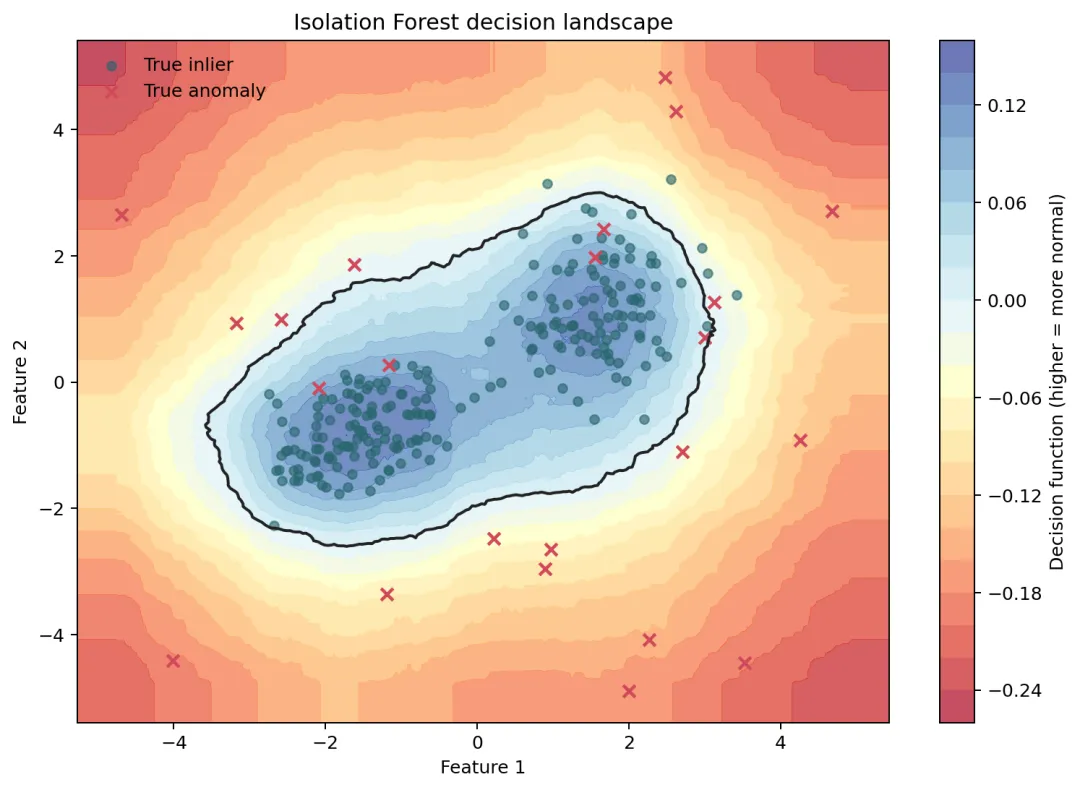
黑色曲线是 decision_function=0 的决策边界。蓝色区域的正常度较高,外围红色区域更容易被随机切分迅速孤立。大部分红色叉号位于边界之外,但几个落在正常簇附近的真实异常没有被分开,说明“稀有”与“异常”并不完全等价。
评估异常排序与阈值表现
# ROC-AUC与平均精确率评价连续异常分数,精确率和召回率评价当前阈值roc_auc = roc_auc_score(y_test, test_anomaly_score)average_precision = average_precision_score(y_test, test_anomaly_score)precision = precision_score(y_test, test_pred)recall = recall_score(y_test, test_pred)f1 = f1_score(y_test, test_pred)print(f”roc_auc: {roc_auc:.3f}”)print(f”average_precision: {average_precision:.3f}”)print(f”precision_at_threshold: {precision:.3f}”)print(f”recall_at_threshold: {recall:.3f}”)print(f”f1_at_threshold: {f1:.3f}”)# 分数分布用于理解阈值位置,虚线右侧会被模型标记为异常pr_precision, pr_recall, pr_thresholds = precision_recall_curve(y_test, test_anomaly_score)fig, axes = plt.subplots(1, 2, figsize=(10.2, 4.6))axes[0].hist(test_anomaly_score[y_test == 0], bins=24, alpha=0.62,color=”#28666E”, label=”True inlier”)axes[0].hist(test_anomaly_score[y_test == 1], bins=18, alpha=0.68,color=”#D1495B”, label=”True anomaly”)axes[0].axvline(score_threshold, color=”#222222”, linestyle=”--”,linewidth=1.7, label=”Model threshold”)axes[0].set(title=”Anomaly score distributions”,xlabel=”Anomaly score (higher = more abnormal)”, ylabel=”Count”)axes[0].legend(frameon=False)# PR曲线更直接呈现稀少异常类别中精确率与召回率的取舍axes[1].plot(pr_recall, pr_precision, color=”#7A5195”, linewidth=2.2)axes[1].scatter([recall], [precision], color=”#D1495B”, s=55,label=”Current threshold”, zorder=3)axes[1].axhline(y_test.mean(), color=”#777777”, linestyle=”:”,label=”Anomaly prevalence”)axes[1].set(title=”Precision-recall trade-off”, xlabel=”Recall”, ylabel=”Precision”,xlim=(0, 1.02), ylim=(0, 1.02))axes[1].legend(frameon=False, loc=”lower left”)fig.tight_layout()fig.savefig(”isolation_forest_diagnostics.png”, dpi=180,bbox_inches=”tight”, facecolor=”white”)plt.close(fig)
输出:
roc_auc: 0.958average_precision: 0.832precision_at_threshold: 0.783recall_at_threshold: 0.783f1_at_threshold: 0.783
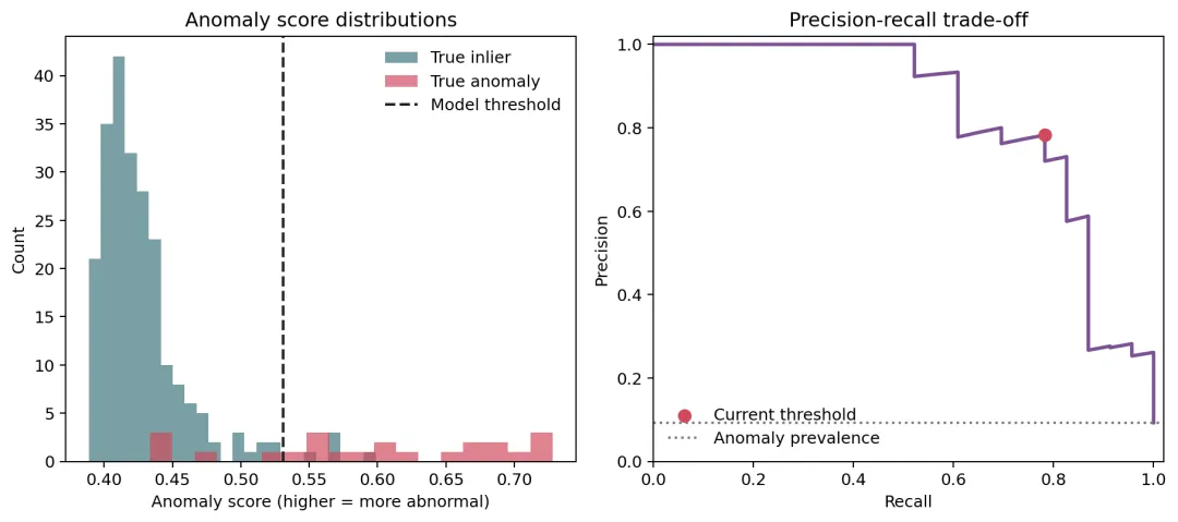
左图显示大部分异常分数位于正常样本右侧,但在 0.44–0.57 附近仍有重叠。虚线阈值为 0.531;阈值右侧被判为异常。右图中的红点是当前阈值位置,改变阈值就会沿着 PR 曲线移动,而不是改变模型已经学到的排序。
结果解释
测试集 ROC-AUC 为 0.958,说明随机抽取一个异常和一个正常样本时,异常获得更高异常分数的概率很高。平均精确率为 0.832,也明显高于测试集约 9.3% 的异常基线比例。两个指标共同说明连续分数具有较好的排序能力,但不能证明每个异常都能被识别。
在 9% 的 contamination 假设下,模型把 23 个测试样本标为异常。精确率 0.783 表示这些报警中约 78.3% 是真实异常;召回率 0.783 表示约 78.3% 的真实异常被找出。两者恰好相等是本次固定模拟与阈值产生的结果,不是孤立森林的一般性质。
实际项目中,阈值应由业务代价决定。如果漏掉异常的损失更大,可以降低阈值以提高召回率;如果人工审核资源紧张,可以提高阈值以增加精确率。contamination 最好来自历史报警率、抽样审计或容量约束,而不是为了让测试集指标最好看而反复试值。
结论
孤立森林把异常检测转化为“一个样本需要多少次随机切分才能被孤立”。它不要求异常标签,也不需要预先假设正常数据是单个圆形簇,适合用作大批量记录的初筛模型。
真正落地时,应保留连续异常分数,不要只保存 0/1 标签;同时监控分数分布和报警率随时间的变化。模型发现的是统计上的稀有结构,不一定等于错误、欺诈或故障,最终仍要结合领域规则与人工复核。
本文结果来自固定随机种子的二维模拟数据,只用于说明模型、阈值和评估流程。高维数据中的无关特征、类别变量编码、概念漂移和群体差异都可能改变实际表现。