【生信分析】Python-10.功能富集分析-超几何分布检验解读高通量实验筛选出的基因列表
- 2026-09-15 13:40:27

生物信息学分析(生信分析)是结合生物学、计算机科学和统计学,对生物数据进行处理、挖掘和解释的多学科领域。其核心思想是通过计算手段从海量数据(如基因组、转录组、蛋白质组数据)中提取生物学洞见,从而解决疾病机制、基因功能、进化关系等问题。

10. 功能富集分析-超几何分布检验
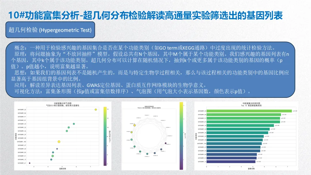
概念:一种用于检验感兴趣的基因集合是否在某个功能类别(如GO term或KEGG通路)中过度出现的统计检验方法。
原理:将问题抽象为“不放回抽样”模型。假设总共有N个基因,其中M个属于某个功能类别。我们感兴趣的基因列表有n个基因,其中k个属于该功能类别。超几何分布可以计算在随机情况下,抽到k个或更多属于该功能类别的基因的概率(p值)。p值越小,说明富集越显著。
思想:如果我们的基因列表不是随机产生的,而是与特定生物学过程相关,那么与该过程相关的功能类别中的基因比例应显著高于基因组背景中的比例。
应用:解读差异表达基因列表、GWAS定位基因、蛋白质互作网络模块的生物学意义。
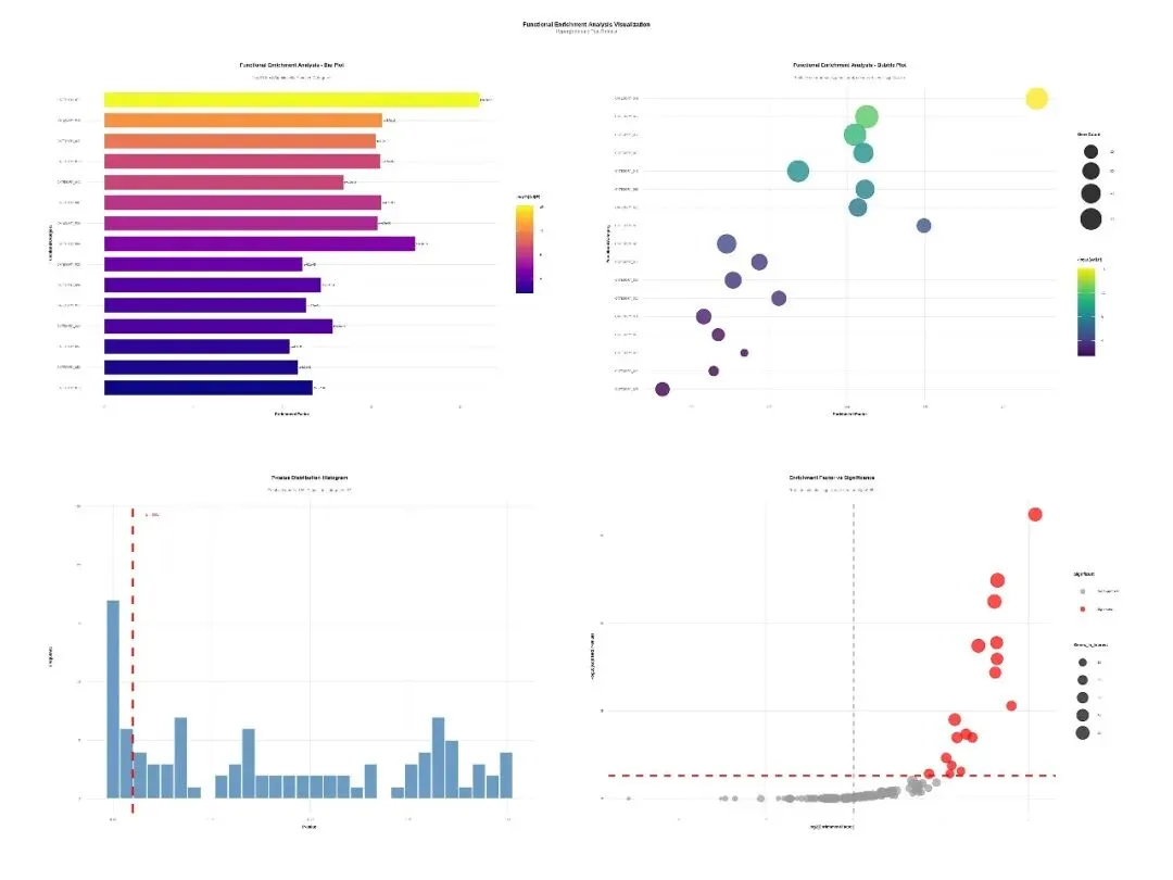
可视化方法:富集条形图(按p值或富集倍数排序)、气泡图(用气泡大小表示基因数,颜色表示p值)。
生信分析可按照分析目的和数据层次分为以下几个主要方面:
1. 序列分析
2. 结构分析
3. 比较基因组学与进化分析
4. 转录组学与基因表达分析
5. 表观基因组学
6. 蛋白质组学与互作网络
7. 单细胞组学
8. 整合多组学与系统生物学
9. 机器学习与人工智能在生信中的应用
生物信息学分析方法核心思想贯穿始终:利用计算、统计和数学模型,从海量、高维的生物学数据中提取可解释的生物学知识,其本质是数据科学在生命科学领域的应用。以下基于常见研究流程,将生信分析方法分为 5 个主要方面,并详细介绍各类方法的概念、原理、思想、应用及可视化方式。
# pip install numpy pandas scipy statsmodels matplotlib seaborn openpyxl python-docx"""功能富集分析:超几何检验流程版本:Python 3.12结果保存到:桌面10_HT-Results文件夹"""# ============================================================================# 1. 导入必要的库# ============================================================================import osimport sysimport numpy as npimport pandas as pdimport randomimport mathfrom datetime import datetimefrom typing import Dict, List, Any, Tupleimport warningswarnings.filterwarnings('ignore')# 统计检验库from scipy import statsfrom scipy.special import combimport statsmodels.stats.multitest as multitest# 数据可视化库import matplotlib.pyplot as pltimport seaborn as snsimport matplotlib.cm as cmfrom matplotlib.patches import Patchfrom matplotlib.lines import Line2D# 报告生成库from openpyxl import Workbookfrom openpyxl.styles import Font, PatternFill, Border, Side, Alignmentfrom openpyxl.utils import get_column_letterfrom docx import Documentfrom docx.shared import Inches, Pt, RGBColorfrom docx.enum.text import WD_ALIGN_PARAGRAPHfrom docx.enum.table import WD_TABLE_ALIGNMENT# ============================================================================# 2. 创建结果文件夹结构# ============================================================================def create_directory_structure():"""创建结果文件夹结构"""# 获取桌面路径 desktop_path = os.path.join(os.path.expanduser("~"), "Desktop") base_dir = os.path.join(desktop_path, "10_HT_Results")# 子文件夹列表 sub_dirs = ["Data", "Plots", "Tables", "Reports"]if not os.path.exists(base_dir): os.makedirs(base_dir)print(f"✓ 创建主文件夹: {base_dir}")for sub_dir in sub_dirs: dir_path = os.path.join(base_dir, sub_dir)if not os.path.exists(dir_path): os.makedirs(dir_path)print(f"✓ 创建子文件夹: {dir_path}")return base_dir# ============================================================================# 3. 模拟数据生成# ============================================================================class DataSimulator:"""数据模拟器""" def __init__(self, seed=12345):"""初始化模拟器""" np.random.seed(seed) random.seed(seed) def simulate_background_genes(self, n_total_genes=20000):"""模拟背景基因集""" background_genes = [f"GENE{i + 1}"for i in range(n_total_genes)]return background_genes def simulate_functional_categories(self, background_genes, n_categories=100):"""模拟功能类别(如GO/KEGG)""" category_names = [f"CATEGORY_{i + 1}"for i in range(n_categories)] category_gene_lists = {}for i, category_name in enumerate(category_names):# 每个类别包含约100-500个基因 n_genes_in_category = np.random.randint(100, 500) selected_genes = np.random.choice( background_genes, size=min(n_genes_in_category, len(background_genes)), replace=False ) category_gene_lists[category_name] = list(selected_genes)return category_names, category_gene_lists def simulate_interest_genes(self, background_genes, category_gene_lists, n_interest_genes=500, n_enriched_categories=15, bias_factor=3):"""模拟感兴趣的基因列表(如差异表达基因)""" category_names = list(category_gene_lists.keys())# 选择富集类别 enriched_categories = np.random.choice( range(len(category_names)), size=n_enriched_categories, replace=False ) interest_genes = set()# 为每个类别选择基因for cat_idx in range(len(category_names)): category_name = category_names[cat_idx] category_genes = category_gene_lists[category_name]if cat_idx in enriched_categories:# 对于富集类别,取更多基因 n_to_select = min( int(len(category_genes) * 0.3 * bias_factor), len(category_genes) )else:# 对于非富集类别,随机选取少量基因 n_to_select = np.random.randint(1, 6)if n_to_select > 0 and len(category_genes) > 0: n_to_select = min(n_to_select, len(category_genes)) selected = np.random.choice(category_genes, size=n_to_select, replace=False) interest_genes.update(selected)# 确保不重复并补充到指定数量 interest_genes = list(interest_genes)if len(interest_genes) < n_interest_genes:# 补充额外基因 remaining_genes = list(set(background_genes) - set(interest_genes)) n_needed = n_interest_genes - len(interest_genes)if len(remaining_genes) >= n_needed: additional_genes = np.random.choice(remaining_genes, size=n_needed, replace=False) interest_genes.extend(additional_genes)else: interest_genes.extend(remaining_genes)else:# 如果基因太多,随机选择指定数量 interest_genes = np.random.choice(interest_genes, size=n_interest_genes, replace=False)return list(interest_genes)# ============================================================================# 4. 超几何分布检验实现# ============================================================================class HypergeometricTest:"""超几何检验分析器""" @staticmethod def perform_test(interest_genes, category_gene_lists, background_genes):""" 执行超几何分布检验 参数: interest_genes: 感兴趣的基因列表 category_gene_lists: 字典,键为类别名,值为该类别中的基因列表 background_genes: 背景基因列表 返回: DataFrame,包含检验结果 """ results = [] N = len(background_genes) # 总基因数 n = len(interest_genes) # 感兴趣基因数for category_name, category_genes in category_gene_lists.items(): M = len(category_genes) # 类别中基因数# 计算交集 overlap_genes = list(set(interest_genes) & set(category_genes)) k = len(overlap_genes) # 交集基因数if M > 0 and k > 0:# 超几何分布检验# 计算p值: P(X >= k) = 1 - P(X <= k-1) p_value = 1 - stats.hypergeom.cdf(k - 1, N, M, n)# 计算富集因子if (M / N) > 0: enrichment_factor = (k / n) / (M / N)else: enrichment_factor = np.nan# 期望值 expected = n * (M / N) results.append({"Category": category_name,"Genes_In_Category": M,"Genes_In_Interest": k,"Expected": round(expected, 2),"Enrichment_Factor": round(enrichment_factor, 3),"P_Value": p_value,"Overlap_Genes": ";".join(overlap_genes) })# 转换为DataFrame results_df = pd.DataFrame(results)if not results_df.empty:# 多重检验校正 (Benjamini-Hochberg方法) results_df["P_Adjust"] = multitest.multipletests( results_df["P_Value"], method='fdr_bh' )[1]# 计算-log10(P值) results_df["log10_P"] = -np.log10(results_df["P_Value"]) results_df["log10_P_Adjust"] = -np.log10(results_df["P_Adjust"])# 添加显著性标记 results_df["Significance"] = results_df["P_Adjust"].apply( lambda x: "***"if x < 0.001 else ("**"if x < 0.01 else ("*"if x < 0.05 else"")) )# 按P值排序 results_df = results_df.sort_values("P_Value")return results_df @staticmethod def calculate_enrichment_factor(k, n, M, N):"""计算富集因子"""if M == 0 or N == 0:return np.nan observed_ratio = k / n if n > 0 else 0 expected_ratio = M / Nreturn observed_ratio / expected_ratio if expected_ratio > 0 else np.nan @staticmethod def hypergeometric_p_value(k, M, N, n):"""计算超几何检验p值"""# P(X >= k) = 1 - P(X <= k-1)return 1 - stats.hypergeom.cdf(k - 1, N, M, n)# ============================================================================# 5. 结果保存器# ============================================================================class ResultsSaver:"""结果保存器""" @staticmethod def save_results(results_df, significant_results, background_genes, interest_genes, output_dir):"""保存所有结果"""# 保存完整结果 full_results_path = os.path.join(output_dir, "Data", "hypergeometric_enrichment_full_results.csv") results_df.to_csv(full_results_path, index=False, encoding='utf-8-sig')print(f"✓ 完整结果已保存: {full_results_path}")# 保存显著结果if not significant_results.empty: significant_path = os.path.join(output_dir, "Data", "hypergeometric_enrichment_significant_results.csv") significant_results.to_csv(significant_path, index=False, encoding='utf-8-sig')print(f"✓ 显著结果已保存: {significant_path}")# 保存背景基因列表 bg_genes_path = os.path.join(output_dir, "Data", "background_genes.txt") with open(bg_genes_path, 'w', encoding='utf-8') as f:for gene in background_genes: f.write(f"{gene}\n")print(f"✓ 背景基因列表已保存: {bg_genes_path}")# 保存感兴趣基因列表 interest_genes_path = os.path.join(output_dir, "Data", "interest_genes.txt") with open(interest_genes_path, 'w', encoding='utf-8') as f:for gene in interest_genes: f.write(f"{gene}\n")print(f"✓ 感兴趣基因列表已保存: {interest_genes_path}")# ============================================================================# 6. Excel三线表生成器# ============================================================================class ExcelTableGenerator:"""Excel三线表生成器""" def __init__(self):"""初始化生成器""" pass def create_excel_tables(self, significant_results, output_dir):"""创建Excel三线表"""if significant_results.empty:print("⚠ 无显著结果,跳过Excel表格生成")return None# 准备三线表数据(取前20个最显著的结果) table_data = significant_results.head(20).copy() table_data = table_data[["Category", "Genes_In_Category", "Genes_In_Interest","Expected", "Enrichment_Factor", "P_Value", "P_Adjust", "Significance" ]]# 创建Excel工作簿 wb = Workbook()# 移除默认工作表if'Sheet'in wb.sheetnames: del wb['Sheet']# 1. 添加超几何检验结果表 ws1 = wb.create_sheet(title="超几何检验结果")# 添加标题 ws1.merge_cells('A1:H1') title_cell = ws1['A1'] title_cell.value = "功能富集分析-超几何分布检验结果表" title_cell.font = Font(bold=True, size=14) title_cell.alignment = Alignment(horizontal='center', vertical='center')# 添加列标题 headers = ["功能类别", "类别基因数", "交集基因数", "期望值","富集倍数", "P值", "校正P值", "显著性"]for col_idx, header in enumerate(headers, 1): cell = ws1.cell(row=3, column=col_idx, value=header) cell.font = Font(bold=True) cell.fill = PatternFill(start_color="F2F2F2", end_color="F2F2F2", fill_type="solid") cell.alignment = Alignment(horizontal='center', vertical='center')# 添加数据行for row_idx, row in enumerate(table_data.itertuples(index=False), 4):for col_idx, value in enumerate(row, 1): cell = ws1.cell(row=row_idx, column=col_idx, value=value) cell.alignment = Alignment(horizontal='center', vertical='center')# 设置列宽for col_idx in range(1, len(headers) + 1): col_letter = get_column_letter(col_idx) ws1.column_dimensions[col_letter].width = 15# 2. 添加说明表 ws2 = wb.create_sheet(title="说明") instructions = [ ["项目", "说明"], ["Category", "功能类别名称"], ["Genes_In_Category", "类别中总基因数"], ["Genes_In_Interest", "感兴趣基因中属于该类别的基因数"], ["Expected", "期望基因数"], ["Enrichment_Factor", "富集倍数"], ["P_Value", "原始P值"], ["P_Adjust", "校正后P值"], ["Significance", "显著性标记(*: p<0.05, **: p<0.01, ***: p<0.001)"] ]for row_idx, instruction in enumerate(instructions, 1):for col_idx, value in enumerate(instruction, 1): cell = ws2.cell(row=row_idx, column=col_idx, value=value) cell.alignment = Alignment(horizontal='left', vertical='center')if row_idx == 1: cell.font = Font(bold=True) cell.fill = PatternFill(start_color="F2F2F2", end_color="F2F2F2", fill_type="solid")# 设置列宽 ws2.column_dimensions['A'].width = 20 ws2.column_dimensions['B'].width = 40# 保存Excel文件 excel_path = os.path.join(output_dir, "Tables", "hypergeometric_enrichment_results.xlsx") wb.save(excel_path)print(f"✓ Excel三线表已保存: {excel_path}")return excel_path# ============================================================================# 7. 可视化分析# ============================================================================class VisualizationGenerator:"""可视化图表生成器""" def __init__(self, output_dir):"""初始化可视化生成器""" self.output_dir = output_dir self.set_matplotlib_style() def set_matplotlib_style(self):"""设置matplotlib样式""" plt.style.use('seaborn-v0_8-whitegrid') sns.set_palette("husl")# 设置中文字体(如果系统支持) try: plt.rcParams['font.sans-serif'] = ['SimHei', 'Arial'] plt.rcParams['axes.unicode_minus'] = False except: pass plt.rcParams.update({'figure.figsize': (10, 6),'figure.dpi': 300,'savefig.dpi': 300,'savefig.bbox': 'tight','savefig.pad_inches': 0.1,'font.size': 12,'axes.titlesize': 16,'axes.labelsize': 14,'xtick.labelsize': 12,'ytick.labelsize': 12,'legend.fontsize': 12,'figure.titlesize': 18,'figure.titleweight': 'bold' }) def plot_bar_enrichment(self, significant_results, n_top=15, save=True):"""绘制富集条形图"""if significant_results.empty:print("⚠ 无显著结果,跳过条形图生成")return None# 准备数据 plot_data = significant_results.head(n_top).copy() plot_data = plot_data.sort_values("Enrichment_Factor", ascending=True) plot_data["Category"] = pd.Categorical( plot_data["Category"], categories=plot_data["Category"].tolist(), ordered=True ) fig, ax = plt.subplots(figsize=(12, 8))# 绘制条形图 colors = plt.cm.viridis(np.linspace(0.2, 0.8, len(plot_data))) bars = ax.barh( plot_data["Category"], plot_data["Enrichment_Factor"], color=colors, edgecolor='white', linewidth=1 )# 添加数值标签for i, bar in enumerate(bars): width = bar.get_width() p_value = plot_data.iloc[i]["P_Adjust"]# 格式化p值if p_value < 0.001: p_str = "p<0.001"elif p_value < 0.01: p_str = f"p={p_value:.2e}"else: p_str = f"p={p_value:.3f}" ax.text( width + 0.1, bar.get_y() + bar.get_height() / 2, p_str, ha='left', va='center', fontsize=10, fontweight='bold' )# 设置标签和标题 ax.set_xlabel("富集倍数", fontweight='bold') ax.set_ylabel("功能类别", fontweight='bold') ax.set_title( f"功能富集分析条形图\nTop {n_top} 最显著富集类别", fontsize=16, fontweight='bold' )# 添加网格 ax.grid(True, axis='x', alpha=0.3)# 调整布局 plt.tight_layout()if save: self.save_plot(fig, "01_富集条形图")return fig def plot_bubble_enrichment(self, significant_results, n_top=20, save=True):"""绘制富集气泡图"""if significant_results.empty:print("⚠ 无显著结果,跳过气泡图生成")return None# 准备数据 plot_data = significant_results.head(n_top).copy() plot_data = plot_data.sort_values("Enrichment_Factor", ascending=True) plot_data["Category"] = pd.Categorical( plot_data["Category"], categories=plot_data["Category"].tolist(), ordered=True ) fig, ax = plt.subplots(figsize=(12, 8))# 绘制气泡图 scatter = ax.scatter( plot_data["Enrichment_Factor"], range(len(plot_data)), s=plot_data["Genes_In_Interest"] * 10, # 气泡大小 c=-np.log10(plot_data["P_Adjust"]), # 气泡颜色 cmap='viridis', alpha=0.8, edgecolors='black', linewidth=0.5 )# 添加颜色条 cbar = plt.colorbar(scatter, ax=ax) cbar.set_label('-log10(校正P值)', fontweight='bold')# 设置y轴标签 ax.set_yticks(range(len(plot_data))) ax.set_yticklabels(plot_data["Category"])# 设置标签和标题 ax.set_xlabel("富集倍数", fontweight='bold') ax.set_ylabel("功能类别", fontweight='bold') ax.set_title("功能富集分析气泡图\n气泡大小表示基因数,颜色表示显著性", fontsize=16, fontweight='bold' )# 添加网格 ax.grid(True, axis='x', alpha=0.3)# 调整布局 plt.tight_layout()if save: self.save_plot(fig, "02_富集气泡图")return fig def plot_pvalue_distribution(self, results_df, save=True):"""绘制P值分布直方图"""if results_df.empty:print("⚠ 无结果数据,跳过P值分布图生成")return None fig, ax = plt.subplots(figsize=(12, 8))# 绘制直方图 n_bins = min(30, max(10, len(results_df) // 10)) ax.hist( results_df["P_Value"], bins=n_bins, color='steelblue', edgecolor='white', alpha=0.8 )# 添加阈值线 ax.axvline(x=0.05, color='red', linestyle='--', linewidth=2)# 添加文本标注 n_significant = len(results_df[results_df["P_Adjust"] < 0.05]) ax.text( 0.1, ax.get_ylim()[1] * 0.9, f"p = 0.05\n显著类别数: {n_significant}", color='red', fontsize=12, fontweight='bold' )# 设置标签和标题 ax.set_xlabel("P值", fontweight='bold') ax.set_ylabel("频数", fontweight='bold') ax.set_title( f"P值分布直方图\n总类别数: {len(results_df)} | 显著类别数: {n_significant}", fontsize=16, fontweight='bold' )# 添加网格 ax.grid(True, alpha=0.3)# 调整布局 plt.tight_layout()if save: self.save_plot(fig, "03_P值分布图")return fig def plot_scatter_enrichment(self, results_df, save=True):"""绘制富集倍数与显著性散点图"""if results_df.empty:print("⚠ 无结果数据,跳过散点图生成")return None# 复制数据以避免修改原数据 plot_data = results_df.copy()# 处理富集因子,确保没有0或负值 plot_data["Enrichment_Factor_Adj"] = plot_data["Enrichment_Factor"].copy()# 将小于等于0的值替换为一个很小的正数 min_positive = plot_data[plot_data["Enrichment_Factor"] > 0]["Enrichment_Factor"].min()if pd.isna(min_positive) or min_positive <= 0: min_positive = 0.001 # 默认值 plot_data.loc[plot_data["Enrichment_Factor"] <= 0, "Enrichment_Factor_Adj"] = min_positive / 10# 计算log2富集倍数 plot_data["log2_Enrichment"] = np.log2(plot_data["Enrichment_Factor_Adj"])# 计算-log10校正P值 plot_data["neg_log10_P_Adjust"] = -np.log10(plot_data["P_Adjust"])# 标记显著性 plot_data["Significant"] = plot_data["P_Adjust"] < 0.05 fig, ax = plt.subplots(figsize=(12, 8))# 分离显著和不显著的点 significant_data = plot_data[plot_data["Significant"]] nonsignificant_data = plot_data[~plot_data["Significant"]]# 绘制不显著的点(使用RGB颜色值)if not nonsignificant_data.empty: ax.scatter( nonsignificant_data["log2_Enrichment"], nonsignificant_data["neg_log10_P_Adjust"], c='#999999', # 使用十六进制颜色代码代替 'grey' s=nonsignificant_data["Genes_In_Interest"] * 5, alpha=0.5, edgecolors='black', linewidth=0.5, label='不显著' )# 绘制显著的点(红色)if not significant_data.empty: ax.scatter( significant_data["log2_Enrichment"], significant_data["neg_log10_P_Adjust"], c='#FF0000', # 红色 s=significant_data["Genes_In_Interest"] * 5, alpha=0.7, edgecolors='black', linewidth=0.5, label='显著' )# 添加阈值线 - 使用有效的颜色格式 ax.axhline(y=-np.log10(0.05), color='#FF0000', linestyle='--', linewidth=1.5) # 红色 ax.axvline(x=0, color='#808080', linestyle='--', linewidth=1) # 灰色,使用十六进制# 设置标签和标题 ax.set_xlabel("log2(富集倍数)", fontweight='bold') ax.set_ylabel("-log10(校正P值)", fontweight='bold') ax.set_title("富集倍数与显著性关系图\n红线表示显著性阈值(p=0.05)", fontsize=16, fontweight='bold' )# 添加图例if not significant_data.empty or not nonsignificant_data.empty: ax.legend(loc='best')# 添加网格 ax.grid(True, alpha=0.3)# 调整布局 plt.tight_layout()if save: self.save_plot(fig, "04_富集散点图")return fig def plot_network_enrichment(self, significant_results, n_top=15, save=True):"""绘制富集网络图(模拟)"""if significant_results.empty:print("⚠ 无显著结果,跳过网络图生成")return None# 准备数据 plot_data = significant_results.head(n_top).copy()# 创建模拟网络数据 np.random.seed(42) n_nodes = len(plot_data) angles = np.linspace(0, 2 * np.pi, n_nodes, endpoint=False) radius = 4 network_data = pd.DataFrame({'node': plot_data["Category"],'x': radius * np.cos(angles),'y': radius * np.sin(angles),'size': np.sqrt(plot_data["Genes_In_Interest"]) * 3,'color': -np.log10(plot_data["P_Adjust"]) }) fig, ax = plt.subplots(figsize=(12, 12))# 绘制散点图(节点) scatter = ax.scatter( network_data["x"], network_data["y"], s=network_data["size"] * 30, c=network_data["color"], cmap='viridis', alpha=0.8, edgecolors='black', linewidth=2 )# 添加节点标签for i, row in network_data.iterrows(): ax.text( row["x"] * 1.15, row["y"] * 1.15, row["node"], fontsize=10, ha='center', va='center', fontweight='bold', bbox=dict(boxstyle="round,pad=0.3", facecolor="white", alpha=0.7, edgecolor="none") )# 添加模拟连接线(基于相似性)for i in range(n_nodes):for j in range(i + 1, n_nodes):# 计算两个节点之间的距离 dist = np.sqrt((network_data.iloc[i]["x"] - network_data.iloc[j]["x"]) ** 2 + (network_data.iloc[i]["y"] - network_data.iloc[j]["y"]) ** 2)# 距离较近的节点添加连接线if dist < radius * 1.5: ax.plot( [network_data.iloc[i]["x"], network_data.iloc[j]["x"]], [network_data.iloc[i]["y"], network_data.iloc[j]["y"]], color='#808080', # 灰色,使用十六进制 alpha=0.3, linewidth=1, zorder=0 )# 添加颜色条 cbar = plt.colorbar(scatter, ax=ax) cbar.set_label('-log10(P值)', fontweight='bold')# 设置标题 ax.set_title("富集类别网络图\n节点大小表示基因数量,颜色表示显著性", fontsize=16, fontweight='bold' )# 隐藏坐标轴 ax.set_xticks([]) ax.set_yticks([]) ax.set_xlabel("") ax.set_ylabel("")# 设置边界 ax.set_xlim(-radius * 1.5, radius * 1.5) ax.set_ylim(-radius * 1.5, radius * 1.5)# 设置等比例 ax.set_aspect('equal')# 调整布局 plt.tight_layout()if save: self.save_plot(fig, "05_富集网络图")return fig def create_combined_plot(self, results_df, significant_results, save=True):"""创建组合图形"""if results_df.empty:print("⚠ 无结果数据,跳过组合图生成")return None# 创建2x2的子图布局 fig, axes = plt.subplots(2, 2, figsize=(16, 12))# 1. 富集条形图(左上) ax1 = axes[0, 0]if not significant_results.empty: plot_data = significant_results.head(10).copy() plot_data = plot_data.sort_values("Enrichment_Factor", ascending=True) plot_data["Category"] = pd.Categorical( plot_data["Category"], categories=plot_data["Category"].tolist(), ordered=True ) colors = plt.cm.viridis(np.linspace(0.2, 0.8, len(plot_data))) bars = ax1.barh( plot_data["Category"], plot_data["Enrichment_Factor"], color=colors, edgecolor='white', linewidth=1 ) ax1.set_xlabel("富集倍数", fontweight='bold') ax1.set_ylabel("功能类别", fontweight='bold') ax1.set_title("Top 10 富集类别", fontsize=14, fontweight='bold') ax1.grid(True, axis='x', alpha=0.3)# 2. P值分布直方图(右上) ax2 = axes[0, 1] n_bins = min(20, max(10, len(results_df) // 10)) ax2.hist( results_df["P_Value"], bins=n_bins, color='steelblue', edgecolor='white', alpha=0.8 ) ax2.axvline(x=0.05, color='#FF0000', linestyle='--', linewidth=2) # 红色 n_significant = len(results_df[results_df["P_Adjust"] < 0.05]) ax2.text( 0.1, ax2.get_ylim()[1] * 0.9, f"p=0.05\n显著: {n_significant}", color='#FF0000', # 红色 fontsize=10, fontweight='bold' ) ax2.set_xlabel("P值", fontweight='bold') ax2.set_ylabel("频数", fontweight='bold') ax2.set_title("P值分布", fontsize=14, fontweight='bold') ax2.grid(True, alpha=0.3)# 3. 富集散点图(左下) ax3 = axes[1, 0]if not results_df.empty:# 准备数据 plot_data = results_df.copy() plot_data["Enrichment_Factor_Adj"] = plot_data["Enrichment_Factor"].copy() min_positive = plot_data[plot_data["Enrichment_Factor"] > 0]["Enrichment_Factor"].min()if pd.isna(min_positive) or min_positive <= 0: min_positive = 0.001 plot_data.loc[plot_data["Enrichment_Factor"] <= 0, "Enrichment_Factor_Adj"] = min_positive / 10 plot_data["log2_Enrichment"] = np.log2(plot_data["Enrichment_Factor_Adj"]) plot_data["neg_log10_P_Adjust"] = -np.log10(plot_data["P_Adjust"]) plot_data["Significant"] = plot_data["P_Adjust"] < 0.05# 分离数据 significant_data = plot_data[plot_data["Significant"]] nonsignificant_data = plot_data[~plot_data["Significant"]]# 绘制if not nonsignificant_data.empty: ax3.scatter( nonsignificant_data["log2_Enrichment"], nonsignificant_data["neg_log10_P_Adjust"], c='#999999', # 灰色,十六进制 s=20, alpha=0.5, edgecolors='black', linewidth=0.5 )if not significant_data.empty: ax3.scatter( significant_data["log2_Enrichment"], significant_data["neg_log10_P_Adjust"], c='#FF0000', # 红色 s=30, alpha=0.7, edgecolors='black', linewidth=0.5 ) ax3.axhline(y=-np.log10(0.05), color='#FF0000', linestyle='--', linewidth=1) # 红色 ax3.axvline(x=0, color='#808080', linestyle='--', linewidth=0.5) # 灰色,十六进制 ax3.set_xlabel("log2(富集倍数)", fontweight='bold') ax3.set_ylabel("-log10(校正P值)", fontweight='bold') ax3.set_title("富集倍数 vs 显著性", fontsize=14, fontweight='bold') ax3.grid(True, alpha=0.3)# 4. 富集气泡图(右下) ax4 = axes[1, 1]if not significant_results.empty: plot_data = significant_results.head(15).copy() plot_data = plot_data.sort_values("Enrichment_Factor", ascending=True) plot_data["Category_Short"] = plot_data["Category"].apply(lambda x: x[:15] + "..."if len(x) > 15 else x) plot_data["Category_Short"] = pd.Categorical( plot_data["Category_Short"], categories=plot_data["Category_Short"].tolist(), ordered=True ) scatter = ax4.scatter( plot_data["Enrichment_Factor"], range(len(plot_data)), s=plot_data["Genes_In_Interest"] * 8, c=-np.log10(plot_data["P_Adjust"]), cmap='viridis', alpha=0.8, edgecolors='black', linewidth=0.5 ) ax4.set_yticks(range(len(plot_data))) ax4.set_yticklabels(plot_data["Category_Short"]) ax4.set_xlabel("富集倍数", fontweight='bold') ax4.set_ylabel("功能类别", fontweight='bold') ax4.set_title("富集气泡图", fontsize=14, fontweight='bold') ax4.grid(True, axis='x', alpha=0.3)# 添加总标题 fig.suptitle("功能富集分析综合可视化\n超几何分布检验结果展示", fontsize=20, fontweight='bold', y=0.98 )# 添加页脚 fig.text( 0.5, 0.01, f"分析生成时间: {datetime.now().strftime('%Y-%m-%d %H:%M:%S')} | 总类别数: {len(results_df)} | 显著类别数: {n_significant}", ha='center', fontsize=10, style='italic' )# 调整布局 plt.tight_layout(rect=[0, 0.05, 1, 0.95])if save: self.save_plot(fig, "06_组合图形", width=16, height=12)return fig def save_plot(self, fig, filename_base, width=12, height=8):"""保存图形到多种格式"""# JPG格式 jpg_file = os.path.join(self.output_dir, "Plots", f"{filename_base}.jpg") fig.savefig(jpg_file, dpi=300, bbox_inches='tight', facecolor='white')# PNG格式 png_file = os.path.join(self.output_dir, "Plots", f"{filename_base}.png") fig.savefig(png_file, dpi=300, bbox_inches='tight', facecolor='white')# PDF格式 pdf_file = os.path.join(self.output_dir, "Plots", f"{filename_base}.pdf") fig.savefig(pdf_file, bbox_inches='tight', facecolor='white')print(f" 已保存: {filename_base} (JPG, PNG, PDF)") plt.close(fig)# ============================================================================# 8. Word报告生成器# ============================================================================class WordReportGenerator:"""Word报告生成器""" def __init__(self, output_dir):"""初始化报告生成器""" self.output_dir = output_dir def create_report(self, results_df, significant_results, background_genes, interest_genes, analysis_params):"""创建Word报告"""# 创建Word文档 doc = Document()# 添加标题 title = doc.add_heading('功能富集分析报告', 0) title.alignment = WD_ALIGN_PARAGRAPH.CENTER# 添加时间戳 timestamp = doc.add_paragraph(f'生成时间: {datetime.now().strftime("%Y年%m月%d日 %H:%M:%S")}') timestamp.alignment = WD_ALIGN_PARAGRAPH.CENTER# 添加空行 doc.add_paragraph()# 1. 分析概述 doc.add_heading('1. 分析概述', level=1) doc.add_paragraph('本报告展示了基于超几何分布检验的功能富集分析结果。') analysis_info = doc.add_paragraph() analysis_info.add_run('分析参数:').bold = True analysis_info.add_run(f'\n - 背景基因总数: {analysis_params["n_total_genes"]}') analysis_info.add_run(f'\n - 感兴趣基因数: {analysis_params["n_interest_genes"]}') analysis_info.add_run(f'\n - 功能类别数: {analysis_params["n_categories"]}') analysis_info.add_run(f'\n - 显著富集类别数 (P_Adjust < 0.05): {len(significant_results)}') doc.add_paragraph()# 2. 方法学 doc.add_heading('2. 方法学', level=1) doc.add_paragraph('超几何分布检验是一种用于检验感兴趣的基因集合是否在某个功能类别中过度出现的统计方法。') method = doc.add_paragraph() method.add_run('计算公式:P = 1 - Σ(i=0 to k-1) [C(M,i) * C(N-M,n-i) / C(N,n)]').italic = True method.add_run('\n其中:') method.add_run('\n - N: 总基因数') method.add_run('\n - M: 功能类别中的基因数') method.add_run('\n - n: 感兴趣基因数') method.add_run('\n - k: 感兴趣基因中属于该功能类别的基因数') method.add_run('\n使用BH方法进行多重检验校正。') doc.add_paragraph()# 3. 结果摘要 doc.add_heading('3. 结果摘要', level=1) doc.add_paragraph(f'共发现 {len(significant_results)} 个显著富集的功能类别(P_Adjust < 0.05)。')if not significant_results.empty:# 添加前10个显著结果表格 doc.add_heading('表1:前10个最显著富集的功能类别', level=2)# 创建表格 summary_table = significant_results.head(10).copy() table = doc.add_table(rows=len(summary_table) + 1, cols=6) table.style = 'Light Grid Accent 1'# 设置表头 headers = ["功能类别", "基因数", "富集倍数", "P值", "校正P值", "显著性"]for i, header in enumerate(headers): cell = table.cell(0, i) cell.text = header cell.paragraphs[0].runs[0].font.bold = True# 填充数据for row_idx, (_, row) in enumerate(summary_table.iterrows(), 1): table.cell(row_idx, 0).text = str(row["Category"]) table.cell(row_idx, 1).text = str(row["Genes_In_Interest"]) table.cell(row_idx, 2).text = f"{row['Enrichment_Factor']:.2f}" table.cell(row_idx, 3).text = f"{row['P_Value']:.2e}" table.cell(row_idx, 4).text = f"{row['P_Adjust']:.2e}" table.cell(row_idx, 5).text = str(row["Significance"]) doc.add_paragraph()# 4. 可视化结果 doc.add_heading('4. 可视化结果', level=1)# 4.1 富集条形图 doc.add_heading('4.1 富集条形图', level=2) doc.add_paragraph('条形图展示了富集倍数最高的功能类别,颜色表示显著性水平。')# 插入图片 bar_chart_path = os.path.join(self.output_dir, "Plots", "01_富集条形图.jpg")if os.path.exists(bar_chart_path): try: doc.add_picture(bar_chart_path, width=Inches(6)) doc.add_paragraph('图1:功能富集条形图', style='Caption') except: doc.add_paragraph('(图片加载失败)') doc.add_paragraph()# 4.2 富集气泡图 doc.add_heading('4.2 富集气泡图', level=2) doc.add_paragraph('气泡图中,气泡大小表示重叠基因数,颜色表示显著性水平。') bubble_chart_path = os.path.join(self.output_dir, "Plots", "02_富集气泡图.jpg")if os.path.exists(bubble_chart_path): try: doc.add_picture(bubble_chart_path, width=Inches(6)) doc.add_paragraph('图2:功能富集气泡图', style='Caption') except: doc.add_paragraph('(图片加载失败)') doc.add_paragraph()# 4.3 P值分布 doc.add_heading('4.3 P值分布', level=2) doc.add_paragraph('P值分布图显示了所有功能类别的统计显著性分布情况。') pvalue_chart_path = os.path.join(self.output_dir, "Plots", "03_P值分布图.jpg")if os.path.exists(pvalue_chart_path): try: doc.add_picture(pvalue_chart_path, width=Inches(6)) doc.add_paragraph('图3:P值分布直方图', style='Caption') except: doc.add_paragraph('(图片加载失败)') doc.add_paragraph()# 4.4 富集倍数与显著性关系 doc.add_heading('4.4 富集倍数与显著性关系', level=2) doc.add_paragraph('散点图展示了富集倍数与统计显著性的关系。') scatter_chart_path = os.path.join(self.output_dir, "Plots", "04_富集散点图.jpg")if os.path.exists(scatter_chart_path): try: doc.add_picture(scatter_chart_path, width=Inches(6)) doc.add_paragraph('图4:富集倍数与显著性关系图', style='Caption') except: doc.add_paragraph('(图片加载失败)') doc.add_paragraph()# 5. 结论与讨论 doc.add_heading('5. 结论与讨论', level=1) doc.add_paragraph('基于超几何分布检验的功能富集分析成功识别了多个显著富集的功能类别。') conclusion = doc.add_paragraph() conclusion.add_run('主要发现:').bold = True conclusion.add_run(f'\n 1. 共发现 {len(significant_results)} 个显著富集的功能类别')if not significant_results.empty: max_enrichment = significant_results["Enrichment_Factor"].max() conclusion.add_run(f'\n 2. 最高富集倍数: {max_enrichment:.2f}') conclusion.add_run('\n 3. 富集倍数最高的类别可能代表核心生物学过程') conclusion.add_run('\n 4. 结果可为后续实验验证提供方向') doc.add_paragraph()# 6. 文件清单 doc.add_heading('6. 文件清单', level=1) doc.add_paragraph('生成的文件保存在以下目录中:') file_list = doc.add_paragraph() file_list.add_run(f'主目录: {self.output_dir}').bold = True file_list.add_run('\n ├── Data/: 原始数据和结果文件') file_list.add_run('\n ├── Plots/: 所有可视化图形文件') file_list.add_run('\n └── Tables/: Excel三线表文件') doc.add_paragraph()# 7. 报告结束 doc.add_heading('报告结束', level=1)# 保存Word文档 word_file = os.path.join(self.output_dir, "Reports", "功能富集分析报告.docx") doc.save(word_file)print(f"✓ Word报告已保存: {word_file}")return word_file# ============================================================================# 9. 主程序# ============================================================================def main():"""主程序"""print("=" * 70)print("开始功能富集分析:超几何检验流程...")print("=" * 70)# 1. 创建结果文件夹print("\n=== 创建结果文件夹 ===") results_dir = create_directory_structure()# 2. 模拟数据生成print("\n=== 生成模拟数据 ===") simulator = DataSimulator(seed=12345)# 模拟背景基因集print("模拟背景基因集...") background_genes = simulator.simulate_background_genes(n_total_genes=20000)print(f"✓ 背景基因集生成完成: {len(background_genes)}个基因")# 模拟功能类别print("模拟功能类别...") category_names, category_gene_lists = simulator.simulate_functional_categories( background_genes, n_categories=100 )print(f"✓ 功能类别生成完成: {len(category_names)}个类别")# 模拟感兴趣的基因列表print("模拟感兴趣的基因列表...") interest_genes = simulator.simulate_interest_genes( background_genes, category_gene_lists, n_interest_genes=500, n_enriched_categories=15, bias_factor=3 )print(f"✓ 感兴趣基因列表生成完成: {len(interest_genes)}个基因")# 3. 超几何分布检验print("\n=== 执行超几何分布检验 ===") hypergeom_test = HypergeometricTest() enrichment_results = hypergeom_test.perform_test( interest_genes, category_gene_lists, background_genes )print(f"✓ 超几何检验完成: {len(enrichment_results)}个类别被分析")# 筛选显著结果 significant_results = enrichment_results[enrichment_results["P_Adjust"] < 0.05].copy()print(f"✓ 显著富集类别: {len(significant_results)}个 (P_Adjust < 0.05)")# 4. 保存结果print("\n=== 保存分析结果 ===") saver = ResultsSaver() saver.save_results( enrichment_results, significant_results, background_genes, interest_genes, results_dir )# 5. 创建Excel三线表print("\n=== 创建科研三线表 ===") excel_generator = ExcelTableGenerator() excel_path = excel_generator.create_excel_tables(significant_results, results_dir)# 6. 可视化分析print("\n=== 生成可视化图表 ===") visualizer = VisualizationGenerator(results_dir)# 6.1 生成富集条形图print("6.1 生成富集条形图...") fig1 = visualizer.plot_bar_enrichment(significant_results, n_top=15)# 6.2 生成富集气泡图print("6.2 生成富集气泡图...") fig2 = visualizer.plot_bubble_enrichment(significant_results, n_top=20)# 6.3 生成P值分布图print("6.3 生成P值分布图...") fig3 = visualizer.plot_pvalue_distribution(enrichment_results)# 6.4 生成散点图print("6.4 生成散点图...") fig4 = visualizer.plot_scatter_enrichment(enrichment_results)# 6.5 生成网络图print("6.5 生成网络图...") fig5 = visualizer.plot_network_enrichment(significant_results, n_top=15)# 6.6 生成组合图形print("6.6 生成组合图形...") fig6 = visualizer.create_combined_plot(enrichment_results, significant_results)print(f"✓ 所有图表已保存到: {os.path.join(results_dir, 'Plots/')}")# 7. 创建Word报告print("\n=== 创建Word报告文档 ===")# 准备分析参数 analysis_params = {"n_total_genes": len(background_genes),"n_interest_genes": len(interest_genes),"n_categories": len(category_names) } word_generator = WordReportGenerator(results_dir) word_path = word_generator.create_report( enrichment_results, significant_results, background_genes, interest_genes, analysis_params )# 8. 生成分析摘要print("\n=== 生成分析摘要 ===")if not significant_results.empty: max_enrichment = significant_results["Enrichment_Factor"].max() min_p_value = significant_results["P_Adjust"].min()else: max_enrichment = 0 min_p_value = 1 summary_text = f"""{'=' * 70}{'功能富集分析 - 超几何检验执行摘要'.center(68)}{'=' * 70}分析时间戳: {datetime.now().strftime("%Y-%m-%d %H:%M:%S")}背景基因总数: {len(background_genes)}感兴趣基因数: {len(interest_genes)}功能类别数: {len(category_names)}分析类别数: {len(enrichment_results)}显著富集类别数 (P_Adjust < 0.05): {len(significant_results)}最高富集倍数: {max_enrichment:.2f}最显著P值: {min_p_value:.2e}生成文件: 1. 数据文件 (Data/): • hypergeometric_enrichment_full_results.csv • hypergeometric_enrichment_significant_results.csv • background_genes.txt • interest_genes.txt 2. 表格文件 (Tables/): • hypergeometric_enrichment_results.xlsx 3. 图形文件 (Plots/): • 01_富集条形图.jpg/.png/.pdf • 02_富集气泡图.jpg/.png/.pdf • 03_P值分布图.jpg/.png/.pdf • 04_富集散点图.jpg/.png/.pdf • 05_富集网络图.jpg/.png/.pdf • 06_组合图形.jpg/.png/.pdf 4. 报告文件 (Reports/): • 功能富集分析报告.docx分析成功完成!{'=' * 70}"""print(summary_text)# 保存执行摘要 summary_path = os.path.join(results_dir, "analysis_summary.txt") with open(summary_path, 'w', encoding='utf-8') as f: f.write(summary_text)# 9. 完成信息输出print("\n" + "=" * 70)print("✅ 分析完成!")print("-" * 70)print(f"📁 结果保存位置:{results_dir}")print("-" * 70)print("📊 生成的文件:")print(" 1. 数据文件(Data/):")print(" • hypergeometric_enrichment_full_results.csv")print(" • hypergeometric_enrichment_significant_results.csv")print(" • background_genes.txt")print(" • interest_genes.txt")print("\n 2. 表格文件(Tables/):")print(" • hypergeometric_enrichment_results.xlsx")print("\n 3. 图形文件(Plots/):")print(" • 01_富集条形图.jpg/.png/.pdf")print(" • 02_富集气泡图.jpg/.png/.pdf")print(" • 03_P值分布图.jpg/.png/.pdf")print(" • 04_富集散点图.jpg/.png/.pdf")print(" • 05_富集网络图.jpg/.png/.pdf")print(" • 06_组合图形.jpg/.png/.pdf")print("\n 4. 报告文件:")print(" • 功能富集分析报告.docx")print("-" * 70)print("📈 分析统计:")print(f" • 总分析类别数:{len(enrichment_results)}")print(f" • 显著富集类别数:{len(significant_results)}")print(f" • 最高富集倍数:{max_enrichment:.2f}")print(f" • 最显著P值:{min_p_value:.2e}")print("=" * 70)# ============================================================================# 运行主程序# ============================================================================if __name__ == "__main__": main()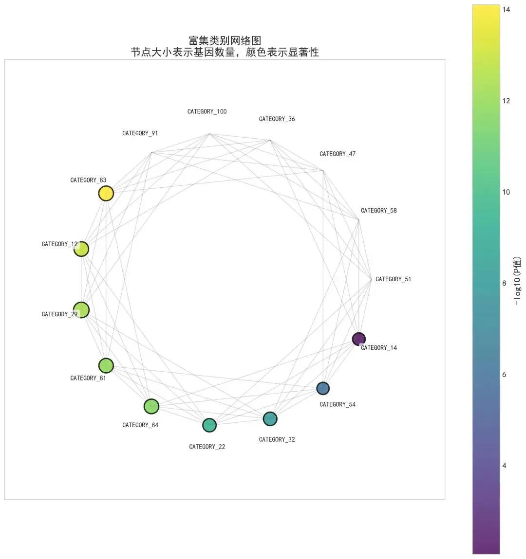
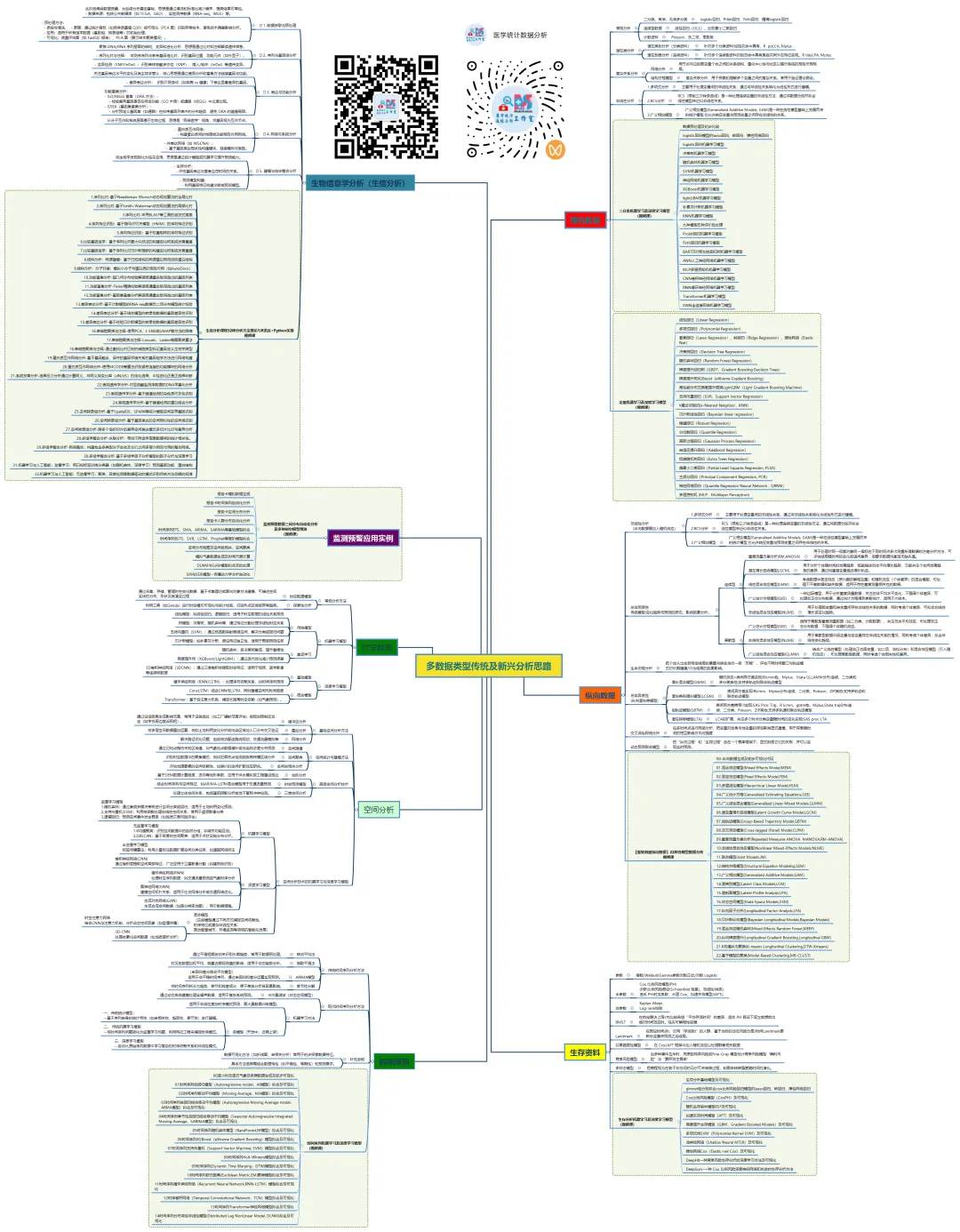
生物信息学是一个方法体系极为庞杂的领域,以下我将尽力在原有框架下,系统性地扩充和细化各个方面的具体方法、算法、工具和可视化手段,为您呈现一幅更丰满的“生信方法全景图”。
1.序列比对-基于Needleman-Wunsch动态规划算法的全局比对
2.序列比对-基于Smith-Waterman动态规划算法的局部比对
3.序列比对-采用BLAST等工具的启发式搜索
4.序列特征识别:基于隐马尔可夫模型(HMM)的序列特征识别
5.序列特征识别:基于权重矩阵的序列特征识别
6.比较基因组学:基于序列比对最大似然法的构建进化树系统发育重建
7.比较基因组学:基于序列比对贝叶斯推断的构建进化树系统发育重建
8.结构分析:同源建模:基于已知结构的同源蛋白预测目标蛋白结构
9.结构分析:分子对接:模拟小分子与蛋白质的相互作用(如AutoDock)
10.功能富集分析-超几何分布检验解读高通量实验筛选出的基因列表
11.功能富集分析-Fisher精确检验解读高通量实验筛选出的基因列表
12.功能富集分析-基因集富集分析解读高通量实验筛选出的基因列表
13.差异表达分析-基于计数模型的RNA-seq数据负二项分布模型统计检验
14.差异表达分析-基于线性模型的转录组数据的基因差异性识别
15.差异表达分析-基于经验贝叶斯模型的转录组数据的基因差异性识别
16.单细胞聚类与注释-使用PCA、t-SNE或UMAP等方法的降维
17.单细胞聚类与注释-Louvain、Leiden等图聚类算法
18.单细胞聚类与注释-通过查找比对已知的细胞类型标记基因定义生物学类型
19.蛋白质互作网络分析-基于基因融合、保守的基因邻接关系的基因组学方法进行网络构建
20.蛋白质互作网络分析-使用MCODE等算法识别紧密连接的功能模块的网络分析
21.系统发育分析-选择压力分析通过计算同义、非同义突变比率(dN/dS)的纯化选择、中性进化还是正选择判断
22.表观遗传学分析-对亚硫酸盐测序数据的DNA甲基化分析
23.表观遗传学分析-基于峰值检测的染色质可及性识别
24.表观遗传学分析-基于峰值检测的蛋白结合分析
25.空间转录组分析-基于SpatialDE、SPARK等统计模型空间变异基因识别
26.空间转录组分析-基于基因表达的空间相似性的空间域识别
27.空间转录组分析-跨多个组织切片的差异空间表达模式多切片比对与差异分析
28.多组学整合分析-关联分析:寻找不同组学层面数据间的统计相关性。
29.多组学整合分析-网络整合:构建包含多类型分子实体及它们之间多层次相互作用的整合网络。
30.多组学整合分析-基于多组学因子分析模型的因子分析与深度学习
31.机器学习与人工智能:监督学习:用已知标签训练分类器(如随机森林、深度学习)预测基因功能、蛋白结构
32.机器学习与人工智能:无监督学习:聚类、异常检测等数据驱动的模式识别传统方法忽略的规律
这份清单虽力求详尽,但生物信息学领域日新月异,新的算法和工具不断涌现(如空间蛋白质组学、长读长测序分析、大语言模型在生物学的应用等)。掌握这些方法的核心思想比记住所有工具名称更重要。在实际研究中,通常需要灵活组合多种方法,形成一条从原始数据到生物学发现的分析流水线。建议的学习路径是:先建立清晰的框架认知(如本回答),然后根据具体研究问题,深入钻研相关的一个或几个子领域。 希望这份扩展版的梳理能为您提供一张有价值的“导航地图”。
医学统计数据分析分享交流SPSS、R语言、Python、ArcGis、Geoda、GraphPad、数据分析图表制作等心得。承接数据分析,论文返修,医学统计,机器学习,生存分析,空间分析,问卷分析,生信分析业务。若有投稿和数据分析代做需求,可以直接联系我,谢谢!

“医学统计数据分析”公众号右下角;
找到“联系作者”,
可加我微信,邀请入粉丝群!

有临床流行病学数据分析
如(t检验、方差分析、χ2检验、logistic回归)、
(重复测量方差分析与配对T检验、ROC曲线)、
(非参数检验、生存分析、样本含量估计)、
(筛检试验:灵敏度、特异度、约登指数等计算)、
(绘制柱状图、散点图、小提琴图、列线图等)、
机器学习、深度学习、生存分析
等需求的同仁们,加入【临床】粉丝群。
疾控,公卫岗位的同仁,可以加一下【公卫】粉丝群,分享生态学研究、空间分析、时间序列、监测数据分析、时空面板技巧等工作科研自动化内容。
有实验室数据分析需求的同仁们,可以加入【生信】粉丝群,交流NCBI(基因序列)、UniProt(蛋白质)、KEGG(通路)、GEO(公共数据集)等公共数据库、基因组学转录组学蛋白组学代谢组学表型组学等数据分析和可视化内容。
或者可扫码直接加微信进群!!!




精品视频课程-“医学统计数据分析”视频号付费合集

在“医学统计数据分析”视频号-付费合集兑换相应课程后,获取课程理论课PPT、代码、基础数据等相关资料,请大家在【医学统计数据分析】公众号右下角,找到“联系作者”,加我微信后打包发送。感谢您的支持!!!
随机文章
-
 10个月宝宝每天需要喝多少奶粉?
- Python办公自动化保姆级教程④:Word文档自动化实战,批量生成合同、填充模板、插入图文、统一格式,彻底解放文案工作
- Python基础数据类型与变量—列表
- 【PhpStorm 2019】PhpStorm 2019全套安装包下载PhpStorm最新完整安装流程与激活指南
- 一个bat文件启动多个python工具
- 一根竖线值十年功力,Linux管道符的8个实战案例,第5个我用了3年
- ARM64 Linux 启动终章(上):全景复盘 ARM64 Linux 启动全貌,从上电到 PID 1
- 想试 Linux 软件,又怕弄乱主系统?我用 Xubuntu 做了一台软件实验机
- [程序员] Linux:msleep vs mdelay
- ChatGPT桌面应用(Linux版,含Codex):Linux原生桌面客户端,AI直接读写本地代码和终端
- 600个Linux命令,可以少用但不能不会.....