Python Logistic回归实战:正则化、概率评估与阈值选择
- 2026-09-08 14:35:20

面对“是否患病”“是否违约”“用户是否流失”这类二分类问题,很多人会先想到 Logistic 回归。它的结构不复杂,却能同时给出类别判断和事件概率,因此至今仍是医学研究、风控与业务分析中的常用基线模型。
容易踩坑的地方,并不是把 LogisticRegression 跑起来,而是后面的几个选择:数值尺度不同的特征要不要标准化,正则化强度怎样确定,AUC 很高是否代表概率也可信,以及默认的 0.5 阈值是否符合实际目标。
这一期用 scikit-learn 自带的乳腺癌诊断数据完成一套可重复的 Logistic 回归流程。我们把恶性样本设为阳性类别,只在训练数据上完成调参与阈值选择,最后再用独立测试集评价模型。
解决的问题
数据包含 569 个样本、30 个连续特征,原始类别为恶性和良性。输入是细胞核图像计算得到的半径、纹理、周长、面积等数值特征,任务是预测样本属于恶性的概率。
本文希望得到三类结果:第一,利用五折交叉验证选择 L2 正则化强度;第二,从训练集的折外预测中确定一个候选分类阈值;第三,在从未参与调参的测试集上同时评价区分度、概率误差、灵敏度和特异度。
这里的案例用于演示建模方法,不构成临床诊断工具。真实临床模型还需要明确纳排标准、处理抽样偏倚,并在独立人群中完成外部验证。
方法原理
Logistic 回归并不直接预测任意实数,而是先建立特征与对数优势之间的线性关系,再通过 Logistic 函数把结果压缩到 0 和 1 之间。得到的数值可以解释为模型给出的阳性概率。概率大于某个阈值时,才进一步转成阳性类别。
scikit-learn 的 LogisticRegression 默认带正则化。本文使用 L2 正则化,它会限制系数过度增大,改善多特征模型的数值稳定性。参数 C 是正则化强度的倒数:C 越小,约束越强;C 越大,模型越接近弱正则化。我们不凭经验拍板,而是用分层五折交叉验证比较一组候选值。
因为正则化直接作用于系数,不同量纲会影响惩罚的公平性,所以标准化应当和模型放在同一条 Pipeline 中。这样每一折验证只使用该折训练部分估计均值和标准差,不会把验证集信息泄漏给预处理步骤。
AUC 衡量模型能否把阳性样本排在阴性样本之前,却不能单独说明预测概率是否准确。为此,本文还查看 PR 曲线、Brier 分数和校准曲线。分类阈值则通过训练集折外概率的 Youden 指数确定,测试标签始终不参与阈值选择。
数据与实现思路
本例使用 load_breast_cancer 内置数据。原始数据将恶性编码为 0、良性编码为 1;为了让灵敏度对应“识别恶性病例的能力”,代码把恶性重新编码为阳性 1。
数据按照类别比例分层划分为 75% 训练集和 25% 测试集。训练集承担特征标准化、正则化调参和候选阈值选择,测试集只在所有选择锁定后使用一次。交叉验证以 ROC AUC 为评分指标,并固定随机种子,保证代码可重复运行。
整个流程分为四段:准备数据、搜索正则化参数、确定阈值并评价、绘制综合诊断图。多段代码在同一个 Python 会话中按顺序执行。
Python完整实战
1. 加载数据并留出独立测试集
import matplotlib.pyplot as pltimport numpy as npimport pandas as pdfrom sklearn.calibration import calibration_curvefrom sklearn.datasets import load_breast_cancerfrom sklearn.linear_model import LogisticRegressionfrom sklearn.metrics import (accuracy_score, average_precision_score, brier_score_loss,confusion_matrix, f1_score, precision_recall_curve,precision_score, recall_score, roc_auc_score, roc_curve)from sklearn.model_selection import (GridSearchCV, StratifiedKFold, cross_val_predict, train_test_split)from sklearn.pipeline import Pipelinefrom sklearn.preprocessing import StandardScaler# 固定随机种子,使数据划分和交叉验证可以重复SEED = 20260816np.random.seed(SEED)# 数据来自scikit-learn内置的乳腺癌诊断数据集data = load_breast_cancer(as_frame=True)X = data.data# 将原始的恶性类别0改成阳性1,便于解释灵敏度y = (data.target == 0).astype(int)# 分层留出25%测试集,测试集不参与任何参数选择X_train, X_test, y_train, y_test = train_test_split(X, y, test_size=0.25, stratify=y, random_state=SEED)print(f”数据维度:{X.shape}”)print(f”恶性/良性:{int(y.sum())}/{int((1-y).sum())}”)print(f”训练集/测试集:{len(X_train)}/{len(X_test)}”)print(f”测试集恶性比例:{y_test.mean():.3f}”)
输出:
数据维度:(569, 30)恶性/良性:212/357训练集/测试集:426/143测试集恶性比例:0.371
2. 用交叉验证选择正则化强度
# 把标准化和Logistic回归封装在同一流水线中,防止信息泄漏pipe = Pipeline([(”scale”, StandardScaler()),(”model”, LogisticRegression(solver=”liblinear”, max_iter=5000, random_state=SEED))])# C越小代表L2正则化越强,在对数尺度上设置候选值param_grid = {”model__C”: [0.01, 0.03, 0.1, 0.3, 1, 3, 10, 30, 100]}# 分层五折保持每折类别比例接近,并以ROC AUC选择参数cv = StratifiedKFold(n_splits=5, shuffle=True, random_state=SEED)search = GridSearchCV(pipe, param_grid=param_grid, scoring=”roc_auc”,cv=cv, n_jobs=1, return_train_score=True)search.fit(X_train, y_train)# 整理每个C的平均验证AUC和折间标准差results = pd.DataFrame(search.cv_results_)cv_summary = pd.DataFrame({”C”: results[”param_model__C”].astype(float),”mean_auc”: results[”mean_test_score”],”sd_auc”: results[”std_test_score”]}).sort_values(”C”)# 误差线展示五折之间的波动,虚线标出最终选择fig, ax = plt.subplots(figsize=(8.5, 5.3), dpi=160)ax.errorbar(cv_summary[”C”], cv_summary[”mean_auc”],yerr=cv_summary[”sd_auc”], marker=”o”,linewidth=2, capsize=4, color=”#2468a2”)ax.axvline(search.best_params_[”model__C”], linestyle=”--”, color=”#d95f02”,label=f”Best C = {search.best_params_['model__C']}”)ax.set_xscale(”log”)ax.set_xlabel(”Inverse regularization strength (C)”)ax.set_ylabel(”5-fold validation ROC AUC”)ax.set_title(”Cross-validated regularization strength”)ax.legend(frameon=False)fig.tight_layout()plt.savefig(”logistic_cv.png”, bbox_inches=”tight”)plt.close()print(f”最佳C:{search.best_params_['model__C']}”)print(f”最佳五折AUC:{search.best_score_:.4f}”)print(cv_summary.sort_values(”mean_auc”, ascending=False).head(3).to_string(index=False, float_format=lambda x: f”{x:.4f}”))
输出:
最佳C:3最佳五折AUC:0.9978C mean_auc sd_auc3.0000 0.9978 0.00251.0000 0.9978 0.002310.0000 0.9976 0.0027
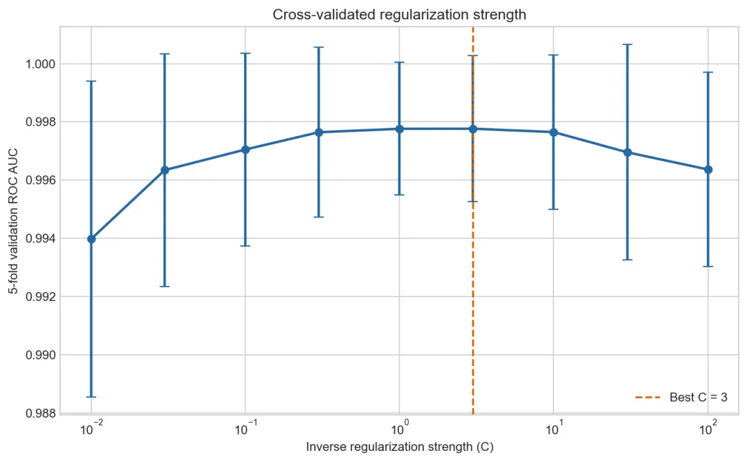
不同 C 的交叉验证 AUC 都较高,说明结论并不依赖某一个极窄的参数点。网格搜索最终选择 C=3;由于 C=1 与其平均 AUC 几乎相同,这里的“最佳”不应被解释成绝对唯一的参数。
3. 用训练集折外概率确定阈值
# 对训练集生成折外概率,每个样本都由未见过它的模型预测oof_prob = cross_val_predict(search.best_estimator_, X_train, y_train,cv=cv, method=”predict_proba”, n_jobs=1)[:, 1]# 在训练集折外ROC上最大化Youden指数,测试集不参与选择fpr_oof, tpr_oof, thresholds = roc_curve(y_train, oof_prob)finite = np.isfinite(thresholds)youden = tpr_oof[finite] - fpr_oof[finite]best_threshold = thresholds[finite][np.argmax(youden)]# 网格搜索对象已经用最佳参数在完整训练集上重新拟合test_prob = search.best_estimator_.predict_proba(X_test)[:, 1]# 同一函数统一计算默认阈值与候选阈值下的分类指标def score_at(threshold):pred = (test_prob >= threshold).astype(int)tn, fp, fn, tp = confusion_matrix(y_test, pred).ravel()return {”accuracy”: accuracy_score(y_test, pred),”precision”: precision_score(y_test, pred),”sensitivity”: recall_score(y_test, pred),”specificity”: tn / (tn + fp),”f1”: f1_score(y_test, pred),”tn”: tn, ”fp”: fp, ”fn”: fn, ”tp”: tp}default_score = score_at(0.5)tuned_score = score_at(best_threshold)roc_auc = roc_auc_score(y_test, test_prob)ap = average_precision_score(y_test, test_prob)brier = brier_score_loss(y_test, test_prob)print(f”折外候选阈值:{best_threshold:.4f}”)print(f”测试集 ROC AUC:{roc_auc:.4f}”)print(f”测试集 AP:{ap:.4f},Brier:{brier:.4f}”)print(f”阈值0.5:灵敏度={default_score['sensitivity']:.4f},特异度={default_score['specificity']:.4f}”)print(f”候选阈值:灵敏度={tuned_score['sensitivity']:.4f},特异度={tuned_score['specificity']:.4f}”)print(f”混淆矩阵 TN/FP/FN/TP:{tuned_score['tn']}/{tuned_score['fp']}/{tuned_score['fn']}/{tuned_score['tp']}”)
输出:
折外候选阈值:0.5228测试集 ROC AUC:0.9841测试集 AP:0.9830,Brier:0.0227阈值0.5:灵敏度=0.9623,特异度=0.9889候选阈值:灵敏度=0.9623,特异度=0.9889混淆矩阵 TN/FP/FN/TP:89/1/2/51
4. 综合检查区分度、校准与阈值权衡
# 提取标准化后的模型系数,绝对值反映线性预测中的相对贡献coef = pd.Series(search.best_estimator_.named_steps[”model”].coef_[0],index=X.columns)top_coef = coef.reindex(coef.abs().sort_values(ascending=False).index).head(6)# 分别计算ROC、PR和分位数分箱校准曲线fpr, tpr, _ = roc_curve(y_test, test_prob)precision, recall, _ = precision_recall_curve(y_test, test_prob)prob_true, prob_pred = calibration_curve(y_test, test_prob, n_bins=8, strategy=”quantile”)# 扫描一组阈值,观察灵敏度、特异度和F1的取舍threshold_grid = np.linspace(0.05, 0.95, 91)threshold_df = pd.DataFrame([{”threshold”: t, **score_at(t)} for t in threshold_grid])# 四个子图分别回答排序、阳性预测、校准和阈值问题fig, axes = plt.subplots(2, 2, figsize=(10.4, 8.2), dpi=160)axes[0, 0].plot(fpr, tpr, color=”#2468a2”, linewidth=2,label=f”AUC = {roc_auc:.3f}”)axes[0, 0].plot([0, 1], [0, 1], ”--”, color=”0.6”)axes[0, 0].set(xlabel=”False positive rate”, ylabel=”True positive rate”,title=”ROC curve”)axes[0, 0].legend(frameon=False)axes[0, 1].plot(recall, precision, color=”#1b9e77”, linewidth=2,label=f”AP = {ap:.3f}”)axes[0, 1].axhline(y_test.mean(), linestyle=”--”, color=”0.6”,label=f”Prevalence = {y_test.mean():.3f}”)axes[0, 1].set(xlabel=”Recall”, ylabel=”Precision”,title=”Precision-recall curve”)axes[0, 1].legend(frameon=False)axes[1, 0].plot(prob_pred, prob_true, marker=”o”,color=”#7570b3”, linewidth=2)axes[1, 0].plot([0, 1], [0, 1], ”--”, color=”0.6”)axes[1, 0].set(xlabel=”Mean predicted probability”,ylabel=”Observed fraction”, title=”Calibration curve”)axes[1, 1].plot(threshold_df[”threshold”], threshold_df[”sensitivity”],label=”Sensitivity”, color=”#d95f02”)axes[1, 1].plot(threshold_df[”threshold”], threshold_df[”specificity”],label=”Specificity”, color=”#1b9e77”)axes[1, 1].plot(threshold_df[”threshold”], threshold_df[”f1”],label=”F1”, color=”#2468a2”)axes[1, 1].axvline(best_threshold, linestyle=”--”, color=”0.25”,label=f”OOF threshold = {best_threshold:.2f}”)axes[1, 1].set(xlabel=”Decision threshold”, ylabel=”Metric”,title=”Threshold trade-offs”)axes[1, 1].legend(frameon=False, fontsize=8)for ax in axes.ravel():ax.set_xlim(left=0)fig.suptitle(”Independent test-set evaluation”, fontsize=14, y=1.01)fig.tight_layout()plt.savefig(”logistic_evaluation.png”, bbox_inches=”tight”)plt.close()print(”绝对系数最大的6个特征:”)for name, value in top_coef.items():print(f”{name}: {value:.4f}”)
输出:
绝对系数最大的6个特征:worst texture: 2.4218worst radius: 1.7390worst area: 1.7367fractal dimension error: -1.5588worst perimeter: 1.3821area error: 1.3008
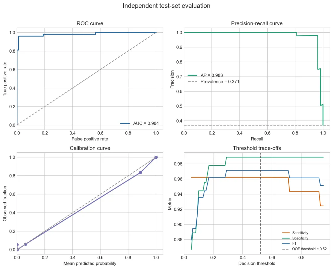
ROC 和 PR 曲线都显示模型具有较强的排序能力。校准曲线大体接近 45 度线,但测试集只有 143 个样本,分箱后的局部起伏不宜过度解读。右下图直观展示了阈值升高时灵敏度下降、特异度上升的常见权衡。
结果解释
五折交叉验证选择 C=3,平均 ROC AUC 为 0.9978。独立测试集 ROC AUC 为 0.9841,平均精确率 AP 为 0.9830,说明模型在本次划分中能较好地区分恶性与良性样本。Brier 分数为 0.0227;它越接近 0,预测概率与实际结局的平方误差越小,但仍应结合校准曲线判断不同概率区间的表现。
训练集折外预测给出的候选阈值为 0.5228。它与默认阈值 0.5 很接近,所以两者在测试集产生了相同分类结果:143 个样本中,正确识别 51 个恶性和 89 个良性,漏掉 2 个恶性,并将 1 个良性判为恶性。对应恶性灵敏度为 0.9623,特异度为 0.9889。
这个结果不能证明 0.5228 是临床最佳阈值。Youden 指数默认同等看待灵敏度和特异度,而现实中的漏诊与误报成本往往不同。若漏诊代价更高,可以有意识地下调阈值来提高灵敏度;若进一步检查昂贵或有创,则需要同时控制误报。阈值应由应用目标决定,而不是由单个指标自动决定。
系数的正负表示对恶性对数优势的方向,绝对值表示在标准化尺度上的相对作用。由于特征之间存在较强相关性,系数不等于独立因果效应,也不宜把排名直接当成生物学重要性排序。正则化还会共同收缩系数,这正是模型获得稳定性所付出的解释代价。
结论
一套可信的 Logistic 回归流程,不应停在 fit 和 predict。标准化与模型要放入同一流水线,正则化参数要在训练数据内部选择,分类阈值也不能借用测试标签反复调整。最后还应把 ROC、PR、概率校准和阈值下的混淆矩阵放在一起看。
Logistic 回归的优势是结构清楚、训练快速、能够输出概率,并且容易作为复杂模型的基线。它的限制同样明确:默认假设特征与对数优势近似线性,相关特征会影响系数稳定性,概率和阈值在新场景中也可能失效。真实应用中还需要检查非线性、交互作用、缺失数据和外部验证。
本例最值得带走的不是某个漂亮分数,而是一条分析纪律:调参和阈值选择都留在训练阶段,独立测试集只负责回答“锁定方案后,模型表现如何”。

随机文章
-
 10个月宝宝每天需要喝多少奶粉?
- 为什么不用linux系统
- Python开发从零开始-50.37-Office 文档处理
- 黄敏珊出席世界机器人大会 Linux 7.3 内核完成版本整合
- 我的实验随笔:Linux篇(6):查看Linux基础信息
- 小白自研日记:Linux 下部署 Node 项目,必用命令与排错思路
- 物业管理微信小程序源码 Python Vue Uniapp
- 【问题解决】基于linux安装blender和brain-coloring,并绘制脑图
- Python进阶教程:15.1_OpenAI 库 —— 全方位使用指南
- 别到处找Linux命令了,这一份够你日常开发
- 【Linux CentOS 7】Linux CentOS 7详细激活版安装教程,新手也能跟着装上