Python画图技巧
- 2026-07-06 21:47:29
import pandas as pd
import matplotlib.pyplot as plt
from matplotlib.dates import DateFormatter
import numpy as np
import os
# 1.字体设置
plt.rcParams.update({
"font.family": "serif",
"font.serif": ["Times New Roman"],
"mathtext.fontset": "stix",
"font.size": 12,
"axes.linewidth": 1.0,
"xtick.direction": "in",
"ytick.direction": "in"
})
# 2. 数据读取与预处理
file_path = r"C:\Users\22076\Desktop\PD2024.csv"
# #这里由于数据集过大因此采用部分数据集,实际使用可以删除掉这部分代码
start_date = "2024-01-01"
end_date = "2024-01-30"
df = pd.read_csv(file_path)
df.columns = df.columns.str.strip()
df["date"] = pd.to_datetime(df["date"])
df.set_index("date", inplace=True)
df_plot = df.loc[start_date:end_date].copy()
df_plot = df_plot.dropna(subset=["PM2.5", "PM10"])
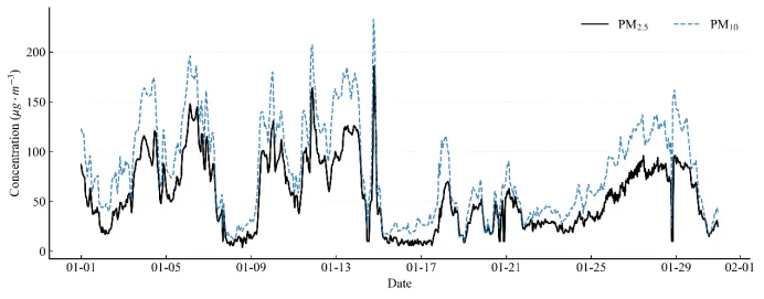
# 3. 绘图执行
fig, ax = plt.subplots(figsize=(10, 4), dpi=300)
# 绘制 PM2.5
ax.plot(
df_plot.index,
df_plot["PM2.5"],
color="black",
linewidth=1.5,
label="PM$_{2.5}$" # LaTeX 下标
)
# 绘制 PM10
ax.plot(
df_plot.index,
df_plot["PM10"],
color="#1f77b4",
linewidth=1.2,
linestyle="--",
alpha=0.9,
label="PM$_{10}$"
)
# 4. 坐标轴
ax.set_ylabel("Concentration ($\mu g \cdot m^{-3}$)")
ax.set_xlabel("Date")
# 时间轴格式化
date_format = DateFormatter("%m-%d")
ax.xaxis.set_major_formatter(date_format)
fig.autofmt_xdate(rotation=0, ha='center')
# 设置图例
ax.legend(frameon=False, loc="upper right", ncol=2) # ncol=2 让图例横向排列,节省垂直空间
ax.spines["top"].set_visible(False)
ax.spines["right"].set_visible(False)
# 添加网格线
ax.grid(axis='y', linestyle=':', alpha=0.3)
plt.tight_layout()
# 5. 图片保存
save_dir = r"C:\Users\22076\Desktop" # 图片保存到桌面
filename_png = os.path.join(save_dir, "PM25_PM10_TimeSeries.png")
plt.savefig(filename_png, dpi=600, bbox_inches='tight')
plt.show()
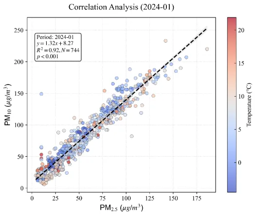
(二)多维散点图
import pandas as pdimport matplotlib.pyplot as pltimport seaborn as snsimport numpy as npimport osfrom scipy import stats# 1. 设置字体plt.rcParams.update({ "font.family": "serif", "font.serif": ["Times New Roman"], "mathtext.fontset": "stix", "font.size": 12, "axes.unicode_minus": False })
# 2. 数据读取与筛选file_path = r"C:\Users\22076\Desktop\PD2024.csv"
#这里由于数据集过大因此采用部分数据集,实际使用可以删除掉这部分代码target_year = 2024target_month = 1 df = pd.read_csv(file_path)df.columns = df.columns.str.strip()df['date'] = pd.to_datetime(df['date'])df_plot = df[(df['date'].dt.year == target_year) & (df['date'].dt.month == target_month)].copy()# 3. 统计分析x = df_plot['PM2.5']y = df_plot['PM10']z = df_plot['气温(℃)']slope, intercept, r_value, p_value, std_err = stats.linregress(x, y)r_squared = r_value ** 2# 统计标签 stats_text = (f'Period: {target_year}-{target_month:02d}\n' f'$y = {slope:.2f}x + {intercept:.2f}$\n' f'$R^2 = {r_squared:.2f}, N = {len(x)}$\n' f'$p < 0.001$')# 4. 绘图fig, ax = plt.subplots(figsize=(8, 6), dpi=600)scatter = ax.scatter(x, y, c=z, cmap='coolwarm', alpha=0.7, edgecolor='k', linewidth=0.3, s=40)# 颜色条cbar = plt.colorbar(scatter, ax=ax)cbar.set_label('Temperature (℃)', fontsize=12)cbar.ax.tick_params(direction='in')# 拟合线x_fit = np.linspace(x.min(), x.max(), 100)y_fit = slope * x_fit + interceptax.plot(x_fit, y_fit, 'k--', linewidth=2, label='Linear Fit')# 95% 置信区间sns.regplot(x=x, y=y, scatter=False, ax=ax, color='gray', ci=95, line_kws={'alpha': 0})# 统计框ax.text(0.05, 0.90, stats_text, transform=ax.transAxes, fontsize=11, verticalalignment='top', bbox=dict(boxstyle='round', facecolor='white', alpha=0.9))# 5. 坐标轴ax.set_xlabel(r'PM$_{2.5}$ ($\mu g/m^3$)', fontsize=14, fontname='Arial') ax.set_ylabel(r'PM$_{10}$ ($\mu g/m^3$)', fontsize=14, fontname='Arial')ax.set_title(f'Correlation Analysis ({target_year}-{target_month:02d})', fontsize=16, pad=15)ax.grid(True, linestyle=':', alpha=0.5)#6.保存图片save_dir = r"C:\Users\22076\Desktop" # 图片保存到桌面filename_png = os.path.join(save_dir, f'Scatter_{target_year}_{target_month:02d}.png')plt.savefig(filename_png, dpi=600, bbox_inches='tight')plt.tight_layout()plt.show()
以上就是本期的全部代码实现。
在实际使用中,记得根据你的数据集来微调数据读取的代码,以及根据你的期刊要求微调 figsize 和 font.size。
代码已开源,从模仿开始,逐渐形成你自己的绘图风格。
如果运行过程中遇到报错,欢迎在后台留言。
本次分享为上海理工大学环境工程2024级硕士研究生张一铭,研究方向:环境大数据应用统计。

