基于Python|完全随机设计的协方差分析图解

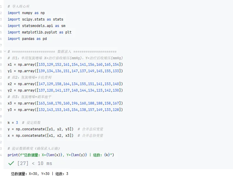
阶段1：环境导入与数据录入，导入核心分析库，录入高血压降压药试验的三组原始数据，合并总数据并验证维度。# 导入核心库import numpy as npimport scipy.stats as statsimport statsmodels.api as smimport matplotlib.pyplot as pltimport pandas as pd# ===================== 数据录入 =====================# 组1：单用氢氯噻嗪 X=治疗前收缩压(mmHg)，Y=治疗后收缩压(mmHg)x1 = np.array([133,129,152,161,154,141,156,160,165,154])y1 = np.array([139,134,136,151,147,137,149,145,155,133])# 组2：氢氯噻嗪+卡托普利x2 = np.array([147,129,158,164,134,155,151,141,153,140])y2 = np.array([137,120,141,137,140,144,134,123,142,130])# 组3：氢氯噻嗪+硝苯地平x3 = np.array([163,168,170,160,196,160,188,188,158,167])y3 = np.array([132,143,153,145,154,138,157,149,133,128])k = 3  # 设定组数y = np.concatenate([y1, y2, y3])  # 合并总应变量x = np.concatenate([x1, x2, x3])  # 合并总协变量# 验证数据维度（确保录入正确）print(f"总数据量：X={len(x)}, Y={len(y)} | 组数：{k}")

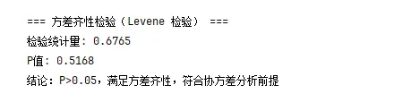
阶段2：方差齐性检验，验证协方差分析的方差齐性前提，笔者换了下，这里与R版稍微有所区别# ===================== 方差齐性检验（Levene检验，鲁棒性更强） =====================levene_result = stats.levene(y1, y2, y3)print("\n=== 方差齐性检验（Levene 检验） ===")print(f"检验统计量: {levene_result.statistic:.4f}")print(f"P值: {levene_result.pvalue:.4f}")# 结果解读if levene_result.pvalue > 0.05:    print("结论：P>0.05，满足方差齐性，符合协方差分析前提")else:    print("结论：P≤0.05，方差不齐，需谨慎使用协方差分析")

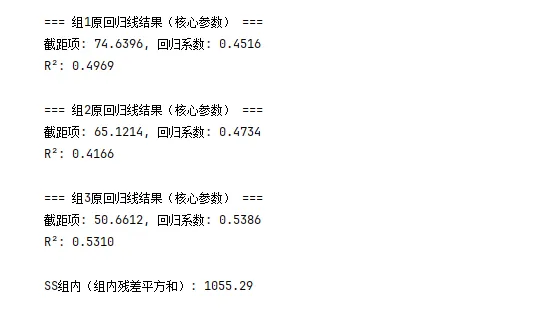
阶段3：拟合各组原回归线+计算SS组内，拟合三组Y对X的原始回归线，获取预测值并计算组内残差平方和# ===================== 定义回归拟合函数（复用） =====================def fit_linear_reg(x_data, y_data):    """    拟合线性回归模型（适配statsmodels）    返回：回归模型、Y预测值    """    x_sm = sm.add_constant(x_data)  # 添加截距项（R的lm默认包含）    model = sm.OLS(y_data, x_sm).fit()  # 普通最小二乘回归    y_hat = model.predict(x_sm)  # 预测值    return model, y_hat# ===================== 拟合各组原回归线 =====================# 组1原回归线model1, y1_hat = fit_linear_reg(x1, y1)print("\n=== 组1原回归线结果（核心参数） ===")print(f"截距项: {model1.params[0]:.4f}, 回归系数: {model1.params[1]:.4f}")print(f"R²: {model1.rsquared:.4f}")# 组2原回归线model2, y2_hat = fit_linear_reg(x2, y2)print("\n=== 组2原回归线结果（核心参数） ===")print(f"截距项: {model2.params[0]:.4f}, 回归系数: {model2.params[1]:.4f}")print(f"R²: {model2.rsquared:.4f}")# 组3原回归线model3, y3_hat = fit_linear_reg(x3, y3)print("\n=== 组3原回归线结果（核心参数） ===")print(f"截距项: {model3.params[0]:.4f}, 回归系数: {model3.params[1]:.4f}")print(f"R²: {model3.rsquared:.4f}")# ===================== 计算SS组内 =====================ss_within = np.sum((y1 - y1_hat)**2) + np.sum((y2 - y2_hat)**2) + np.sum((y3 - y3_hat)**2)ss_within = round(ss_within, 2)  # 保留2位小数print(f"\nSS组内（组内残差平方和）: {ss_within}")

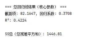
阶段 4：拟合总回归线+计算SS总，拟合合并数据的总回归线，获取总预测值并计算总残差平方和# ===================== 拟合总回归线 =====================model_total, y_hat = fit_linear_reg(x, y)print("\n=== 总回归线结果（核心参数） ===")print(f"截距项: {model_total.params[0]:.4f}, 回归系数: {model_total.params[1]:.4f}")print(f"R²: {model_total.rsquared:.4f}")# ===================== 计算SS总 =====================ss_total = np.sum((y - y_hat)**2)ss_total = round(ss_total, 2)print(f"\nSS总（总残差平方和）: {ss_total}")

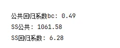
阶段5：拟合平行回归线+计算核心指标，计算公共回归系数，拟合三组平行回归线，计算SS公共、SS回归系数# ===================== 定义离均差计算函数 =====================def calc_lxy_lxx(x_sub, y_sub):    """计算单组的离均差积和(lxy)、离均差平方和(lxx)"""    n = len(x_sub)    lxy = np.sum(x_sub*y_sub) - (np.sum(x_sub)*np.sum(y_sub))/n    lxx = np.sum(x_sub**2) - (np.sum(x_sub))**2/n    return lxy, lxx# ===================== 计算总lxy、总lxx =====================lxy1, lxx1 = calc_lxy_lxx(x1, y1)lxy2, lxx2 = calc_lxy_lxx(x2, y2)lxy3, lxx3 = calc_lxy_lxx(x3, y3)lxy_total = lxy1 + lxy2 + lxy3  # 总离均差积和lxx_total = lxx1 + lxx2 + lxx3  # 总离均差平方和# ===================== 公共回归系数（bc） =====================bc = lxy_total / lxx_totalbc = round(bc, 2)print(f"\n公共回归系数bc: {bc}")  # 与R结果一致（0.49）# ===================== 拟合三组平行回归线 =====================# 公式：y_pxhat = 组Y均值 - bc*组X均值 + bc*Xy1_pxhat = np.mean(y1) - bc*np.mean(x1) + bc*x1y2_pxhat = np.mean(y2) - bc*np.mean(x2) + bc*x2y3_pxhat = np.mean(y3) - bc*np.mean(x3) + bc*x3# ===================== 计算SS公共、SS回归系数 =====================ss_common = np.sum((y1 - y1_pxhat)**2) + np.sum((y2 - y2_pxhat)**2) + np.sum((y3 - y3_pxhat)**2)ss_common = round(ss_common, 2)ss_reg_coef = np.sum((y1_pxhat - y1_hat)**2) + np.sum((y2_pxhat - y2_hat)**2) + np.sum((y3_pxhat - y3_hat)**2)ss_reg_coef = round(ss_reg_coef, 2)print(f"SS公共: {ss_common}")print(f"SS回归系数: {ss_reg_coef}")

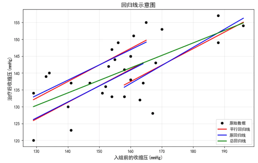
阶段7：回归线可视化，绘制散点图+三组原回归线+三组平行回归线+总回归线# ===================== 绘制回归线示意图（修正版） =====================plt.rcParams['font.sans-serif'] = ['SimHei']  # 解决中文显示问题plt.rcParams['axes.unicode_minus'] = False    # 解决负号显示问题# 基础散点图plt.figure(figsize=(10, 6))plt.scatter(x, y, color='black', s=30, label='原始数据')# 绘制平行回归线（红色）x1_sorted = np.sort(x1)y1_pxhat_sorted = np.mean(y1) - bc*np.mean(x1) + bc*x1_sortedplt.plot(x1_sorted, y1_pxhat_sorted, color='red', linewidth=2, label='平行回归线')x2_sorted = np.sort(x2)y2_pxhat_sorted = np.mean(y2) - bc*np.mean(x2) + bc*x2_sortedplt.plot(x2_sorted, y2_pxhat_sorted, color='red', linewidth=2)x3_sorted = np.sort(x3)y3_pxhat_sorted = np.mean(y3) - bc*np.mean(x3) + bc*x3_sortedplt.plot(x3_sorted, y3_pxhat_sorted, color='red', linewidth=2)# 绘制原回归线（蓝色）y1_hat_sorted = model1.params[0] + model1.params[1]*x1_sortedplt.plot(x1_sorted, y1_hat_sorted, color='blue', linewidth=2, label='原回归线')y2_hat_sorted = model2.params[0] + model2.params[1]*x2_sortedplt.plot(x2_sorted, y2_hat_sorted, color='blue', linewidth=2)y3_hat_sorted = model3.params[0] + model3.params[1]*x3_sortedplt.plot(x3_sorted, y3_hat_sorted, color='blue', linewidth=2)# 绘制总回归线（绿色）x_sorted = np.sort(x)y_hat_sorted = model_total.params[0] + model_total.params[1]*x_sortedplt.plot(x_sorted, y_hat_sorted, color='green', linewidth=2, label='总回归线')# 图表美化（修正图例位置）plt.xlabel('入组前的收缩压(mmHg)', fontsize=12)plt.ylabel('治疗后收缩压(mmHg)', fontsize=12)plt.title('回归线示意图', fontsize=14)plt.legend(loc='lower right', fontsize=10)  # 修正：bottommright → lower rightplt.grid(alpha=0.3)plt.show()

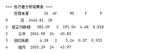
阶段 8：生成协方差分析结果# ===================== 整理基础指标 =====================# 平方和（SS）SS = [ss_total, ss_corrected_mean, ss_common, ss_reg_coef, ss_within]# 自由度（df）df_total = len(x) - 2df_corrected_mean = k - 1df_common = len(x) - k - 1df_reg_coef = k - 1df_within = len(x) - 2*kdf = [df_total, df_corrected_mean, df_common, df_reg_coef, df_within]# 均方（MS）ms_corrected_mean = ss_corrected_mean / df_corrected_meanms_common = round(ss_common / df_common, 2)ms_reg_coef = ss_reg_coef / df_reg_coefms_within = round(ss_within / df_within, 2)MS = ["", round(ms_corrected_mean, 2), ms_common, round(ms_reg_coef, 2), ms_within]# F值f_corrected_mean = round(ms_corrected_mean / (ss_common / df_common), 2)f_parallel = round(ms_reg_coef / (ss_within / df_within), 2)F = ["", f_corrected_mean, "", f_parallel, ""]# P值（F检验）- 修正参数名：df1→dfn，df2→dfdp_corrected_mean = 1 - stats.f.cdf(f_corrected_mean, dfn=df_corrected_mean, dfd=df_common)p_parallel = 1 - stats.f.cdf(f_parallel, dfn=df_reg_coef, dfd=df_within)P = ["", round(p_corrected_mean, 3), "", round(p_parallel, 3), ""]# ===================== 构建结果表 =====================result_df = pd.DataFrame({    "变异来源": ["总", "修正均数间", "公共", "回归系数", "组内"],    "SS": SS,    "df": df,    "MS": MS,    "F": F,    "P": P})print("\n=== 协方差分析结果表 ===")print(result_df)

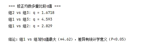
阶段 9：修正均数多重比较（q检验）# ===================== 修正均数多重比较（q检验） =====================# 计算组间lxx（zjlxx）zjx = np.array([np.mean(x1), np.mean(x2), np.mean(x3)])zjlxx = np.sum(zjx**2) - (np.sum(zjx))**2 / len(zjx)# 重新计算组内lxxlxx1 = np.sum(x1**2) - (np.sum(x1))**2 / len(x1)lxx2 = np.sum(x2**2) - (np.sum(x2))**2 / len(x2)lxx3 = np.sum(x3**2) - (np.sum(x3))**2 / len(x3)lxx_total = lxx1 + lxx2 + lxx3# 计算q值ms_within_num = float(ms_within)  # 转换为数值型（避免字符串干扰）q1 = (xzy2 - xzy3) / np.sqrt(ms_within_num/10 * (1 + zjlxx/4127.2))  # 组2vs组3q2 = (xzy1 - xzy3) / np.sqrt(ms_within_num/10 * (1 + zjlxx/(2*4127.2)))  # 组1vs组3q3 = (xzy1 - xzy2) / np.sqrt(ms_within_num/10 * (1 + zjlxx/4127.2))  # 组1vs组2print("\n=== 修正均数多重比较q值 ===")print(f"组2 vs 组3: q = {round(q1, 4)}")print(f"组1 vs 组3: q = {round(q2, 4)}")print(f"组1 vs 组2: q = {round(q3, 4)}")# 结果解读print("\n结论：组1 vs 组3的q值最大（≈4.62），差异有统计学意义（P<0.05）")