想象一下星期五的下午,部门总监扔给你一堆销售数据,要求你在下班之前做出数据报表,并做下分析总结,给出不同销售员业绩统计、不同产品销售额统计、区域销售情况对比分析等,为下周的销售策略做下准备,想想是不是挺崩溃?今天,Henry老师以一种全新的视角带您高效完成这件事,那就是用python做数据分析和可视化洞察。 pip insatll pandas matplotlib openpyxl
pandas:Python的数据处理库
openpyxl:处理Excel文件的利器
matplotlib : 可视化库,绘制各种图表
第一步:使用pandas库进行数据清洗,处理重复和缺失数据
import pandas as pdimport matplotlib.pyplot as pltimport numpy as np# 1. 读取数据df = pd.read_excel('sales_data.xlsx')print(f'原始数据形状:{df.shape}')print(f'原始数据列名:{df.columns.tolist()}')# 2. 查看数据基本信息print('\n数据基本信息:')print(df.info())# 3. 检查缺失值print('\n缺失值统计:')print(df.isnull().sum())# 4. 检查重复值print(f'\n重复订单数:{df.duplicated("订单号").sum()}')# 5. 数据类型转换# 确保销售额是数值型df['销售额'] = pd.to_numeric(df['销售额'], errors='coerce')# 确保日期是日期型df['日期'] = pd.to_datetime(df['日期'])# 6. 处理异常值(比如销售额为负或为0)print(f'\n异常销售额统计:')print(f'销售额<=0的数量:{(df["销售额"] <= 0).sum()}')print(f'销售额>10000的数量:{(df["销售额"] > 10000).sum()}')# 7. 删除异常值(这里简单处理,实际应根据业务规则)df = df[df['销售额'] > 0]df = df[df['销售额'] < 10000] # 假设单笔不超过1万# 8. 清洗后的数据统计print(f'\n清洗后数据形状:{df.shape}')print(f'销售额范围:¥{df["销售额"].min():.2f} - ¥{df["销售额"].max():.2f}')print(f'平均销售额:¥{df["销售额"].mean():.2f}')
第二步:进行不同销售员业绩统计,使用matplotlib库绘制统计图
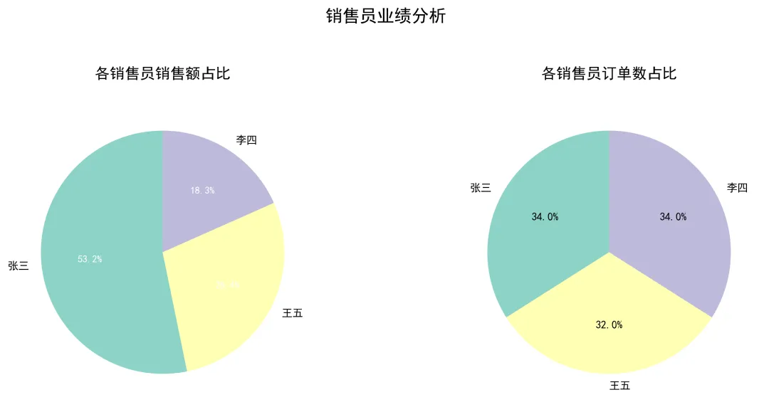
# 1. 按销售员统计销售额salesman_stats = df.groupby('销售员')['销售额'].agg(['sum', 'count', 'mean']).round(2)salesman_stats.columns = ['总销售额', '订单数', '平均客单价']salesman_stats = salesman_stats.sort_values('总销售额', ascending=False)print('\n销售员业绩统计:')print(salesman_stats)# 2. 创建销售员业绩饼图plt.figure(figsize=(12, 5))# 子图1:销售额占比plt.subplot(1, 2, 1)salesman_sums = salesman_stats['总销售额']# 如果销售额太小,合并为"其他"threshold = salesman_sums.sum() * 0.05 # 5%阈值small_salesmen = salesman_sums[salesman_sums < threshold]main_salesmen = salesman_sums[salesman_sums >= threshold]if len(small_salesmen) > 0: plot_data = pd.concat([main_salesmen, pd.Series({'其他': small_salesmen.sum()})])else: plot_data = main_salesmen# 自定义颜色colors = plt.cm.Set3(range(len(plot_data)))# 绘制饼图wedges, texts, autotexts = plt.pie(plot_data.values, labels=plot_data.index, autopct='%1.1f%%', colors=colors, startangle=90)for text in texts: text.set_fontsize(10)for autotext in autotexts: autotext.set_fontsize(9) autotext.set_color('white')plt.title('各销售员销售额占比', fontsize=14, pad=20)# 子图2:订单数占比plt.subplot(1, 2, 2)salesman_counts = salesman_stats['订单数']plt.pie(salesman_counts.values, labels=salesman_counts.index, autopct='%1.1f%%', colors=colors, startangle=90)plt.title('各销售员订单数占比', fontsize=14, pad=20)plt.suptitle('销售员业绩分析', fontsize=16, y=1.05)plt.tight_layout()plt.savefig('01_销售员业绩分析.png', dpi=300, bbox_inches='tight')plt.show()
运行上述程序,可直接得到不同销售员销售业绩对比饼状图,如下:
第三步:不同产品销售额统计,同样使用matplotlib库绘制统计图,代码如下:# 1. 按产品类别统计category_stats = df.groupby('产品类别').agg({ '销售额': ['sum', 'count', 'mean'], '订单号': 'nunique'}).round(2)category_stats.columns = ['总销售额', '订单数', '平均单价', '客户数']category_stats = category_stats.sort_values(('总销售额'), ascending=False)print('\n产品类别销售统计:')print(category_stats)# 2. 按具体产品统计(取前10)product_stats = df.groupby('产品名称').agg({ '销售额': ['sum', 'count'], '产品类别': 'first' # 保留类别信息}).round(2)product_stats.columns = ['总销售额', '销售数量', '产品类别']top10_products = product_stats.nlargest(10, '总销售额')print('\n销售额TOP10产品:')print(top10_products)# 3. 创建产品销售额饼图plt.figure(figsize=(14, 6))# 子图1:产品类别占比plt.subplot(1, 2, 1)category_sums = category_stats['总销售额']colors = plt.cm.Paired(range(len(category_sums)))wedges, texts, autotexts = plt.pie(category_sums.values, labels=category_sums.index, autopct='%1.1f%%', colors=colors, explode=[0.05] * len(category_sums)) # 轻微分离plt.title('各产品类别销售额占比', fontsize=14, pad=20)# 子图2:TOP10产品占比plt.subplot(1, 2, 2)top10_sums = top10_products['总销售额']# 添加"其他"类别other_sum = product_stats['总销售额'].sum() - top10_sums.sum()plot_data = pd.concat([top10_sums, pd.Series({'其他产品': other_sum})])colors2 = plt.cm.tab20(range(len(plot_data)))plt.pie(plot_data.values, labels=plot_data.index, autopct='%1.1f%%', colors=colors2, startangle=90, textprops={'fontsize': 8})plt.title('TOP10产品销售额占比', fontsize=14, pad=20)plt.suptitle('产品销售分析', fontsize=16, y=1.05)plt.tight_layout()plt.savefig('02_产品销售分析.png', dpi=300, bbox_inches='tight')plt.show()
运行上述代码,可以直接得到不同产品销售情况统计饼图,如下: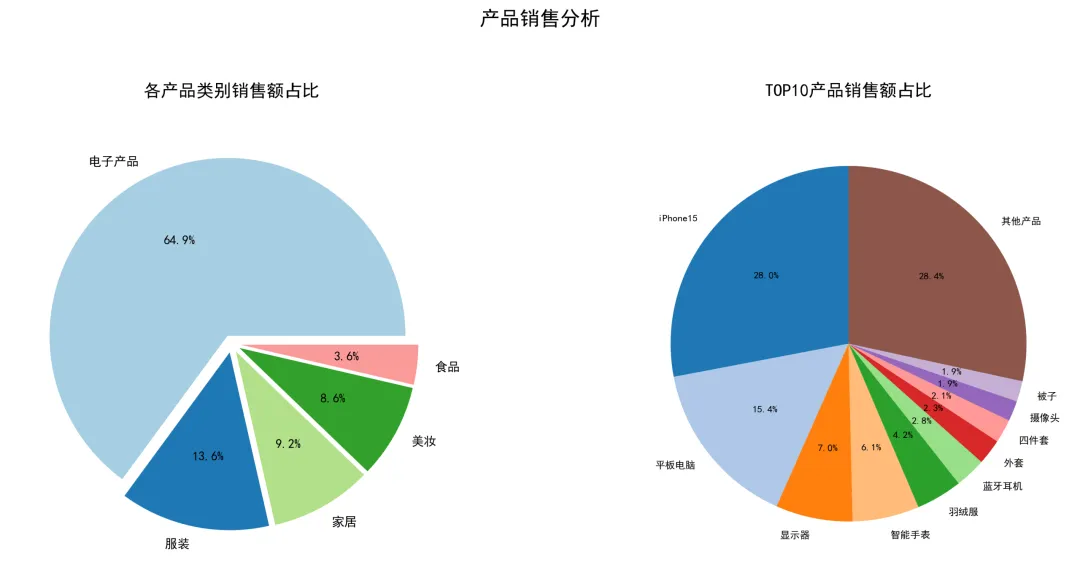
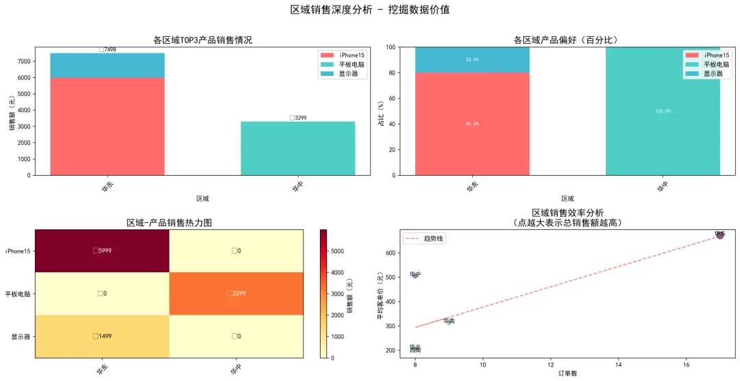
# 1. 选择核心产品进行分析(销售额TOP3的产品)top3_products = product_stats.nlargest(3, '总销售额').index.tolist()print(f'\n选取TOP3产品进行区域对比:{top3_products}')# 2. 创建区域-产品透视表pivot_table = pd.pivot_table( df[df['产品名称'].isin(top3_products)], # 只取TOP3产品 values='销售额', index='区域', columns='产品名称', aggfunc='sum', fill_value=0).round(2)# 添加总计列pivot_table['总计'] = pivot_table.sum(axis=1)pivot_table = pivot_table.sort_values('总计', ascending=False)print('\n各区域TOP3产品销售情况(销售额):')print(pivot_table)# 3. 计算各区域的产品偏好(各产品销售额占比)product_ratio = pivot_table[top3_products].div(pivot_table['总计'], axis=0) * 100product_ratio = product_ratio.round(1)print('\n各区域产品偏好(%):')print(product_ratio)# 4. 绘制区域对比柱状图plt.figure(figsize=(16, 8))# 子图1:区域产品销售额对比(堆叠柱状图)plt.subplot(2, 2, 1)x = range(len(pivot_table.index))bottom = np.zeros(len(pivot_table.index))colors = ['#FF6B6B', '#4ECDC4', '#45B7D1']for i, product in enumerate(top3_products): plt.bar(x, pivot_table[product].values, bottom=bottom, label=product, color=colors[i], width=0.6) bottom += pivot_table[product].valuesplt.xlabel('区域')plt.ylabel('销售额(元)')plt.title('各区域TOP3产品销售情况', fontsize=14)plt.xticks(x, pivot_table.index, rotation=45)plt.legend()# 添加数值标签for i, (idx, row) in enumerate(pivot_table.iterrows()): total = row['总计'] plt.text(i, total + 50, f'¥{total:.0f}', ha='center', va='bottom', fontsize=9)# 子图2:区域产品偏好(百分比堆叠图)plt.subplot(2, 2, 2)bottom = np.zeros(len(product_ratio.index))for i, product in enumerate(top3_products): plt.bar(x, product_ratio[product].values, bottom=bottom, label=product, color=colors[i], width=0.6) bottom += product_ratio[product].valuesplt.xlabel('区域')plt.ylabel('占比(%)')plt.title('各区域产品偏好(百分比)', fontsize=14)plt.xticks(x, product_ratio.index, rotation=45)plt.legend(loc='upper right')# 添加百分比标签for i in range(len(product_ratio.index)): cumulative = 0 for j, product in enumerate(top3_products): value = product_ratio[product].values[i] if value > 5: # 只显示大于5%的标签 plt.text(i, cumulative + value/2, f'{value}%', ha='center', va='center', fontsize=8, color='white') cumulative += value# 子图3:热力图形式(用颜色深浅表示销售额)plt.subplot(2, 2, 3)import seaborn as sns# 如果没有seaborn,用matplotlib模拟heatmap_data = pivot_table[top3_products].Tim = plt.imshow(heatmap_data.values, cmap='YlOrRd', aspect='auto')plt.xticks(range(len(heatmap_data.columns)), heatmap_data.columns, rotation=45)plt.yticks(range(len(heatmap_data.index)), heatmap_data.index)plt.title('区域-产品销售热力图', fontsize=14)# 添加颜色条plt.colorbar(im, label='销售额(元)')# 添加数值标签for i in range(len(heatmap_data.index)): for j in range(len(heatmap_data.columns)): text = plt.text(j, i, f'¥{heatmap_data.values[i, j]:.0f}', ha="center", va="center", color="white" if heatmap_data.values[i, j] > heatmap_data.values.max()/2 else "black")# 子图4:发现数据价值 - 寻找增长机会plt.subplot(2, 2, 4)# 计算各区域的平均客单价和销售效率region_metrics = df.groupby('区域').agg({ '销售额': ['mean', 'sum'], '订单号': 'count'}).round(2)region_metrics.columns = ['平均客单价', '总销售额', '订单数']region_metrics['单均销售额'] = region_metrics['总销售额'] / region_metrics['订单数']# 绘制散点图:订单数 vs 平均客单价plt.scatter(region_metrics['订单数'], region_metrics['平均客单价'], s=region_metrics['总销售额']/100, # 点的大小表示总销售额 alpha=0.6, c=range(len(region_metrics)), cmap='viridis')# 添加区域标签for idx, row in region_metrics.iterrows(): plt.annotate(idx, (row['订单数'], row['平均客单价']), fontsize=9, ha='center')plt.xlabel('订单数')plt.ylabel('平均客单价(元)')plt.title('区域销售效率分析\n(点越大表示总销售额越高)', fontsize=14)# 添加趋势线z = np.polyfit(region_metrics['订单数'], region_metrics['平均客单价'], 1)p = np.poly1d(z)plt.plot(region_metrics['订单数'], p(region_metrics['订单数']), "r--", alpha=0.5, label='趋势线')plt.legend()plt.suptitle('区域销售深度分析 - 挖掘数据价值', fontsize=16, y=1.02)plt.tight_layout()plt.savefig('03_区域销售深度分析.png', dpi=300, bbox_inches='tight')plt.show()
运行上述代码,将会得到各区域Top3产品销售情况,各区域产品偏好(百分比),区域销售热力图等全套数据分析洞察结果。OMG!这也太香了吧!
以前加班到怀疑人生的工作,现在几分钟就搞定了!科技真的是yyds!上面代码直接复制就能用,新手也能轻松上手~
想一起变强的小伙伴:
要完整代码 → 评论区扣"666"
想学Python基础 → 回复"小白上车"
想要更多案例 → 关注我,持续更新!