运行代码后最后展现表格格式如下：csv数据和原代码，关注公众号后私信“power”后回复。

2023年平均碳强度（gCO2eq/kWh）和电力消耗构成（%）

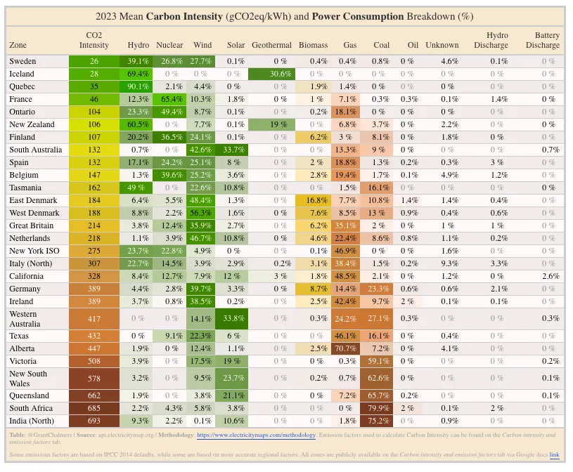
数据来源于Electricity Maps。该项目旨在提供一个免费、开源且透明的全球电力消耗碳强度可视化工具。

在表格中，使用了与碳强度相似的颜色方案，其中绿色代表相对清洁的电力消耗，棕色代表较高排放的消耗。重要的是，电力消耗考虑了邻近电网的进出口，以提供更全面的消耗视图。

虽然Electricity Maps应用程序的实时特性非常出色——但一年的视图有助于消除季节性变化对许多电网碳强度的影响，特别是那些采用高比例可变可再生能源(VRE)的电网。一个很好的例子是加利福尼亚州，它在北半球夏季比冬季明显更清洁。

Electricity Maps屏幕截图，聚焦于凌晨5点的西欧。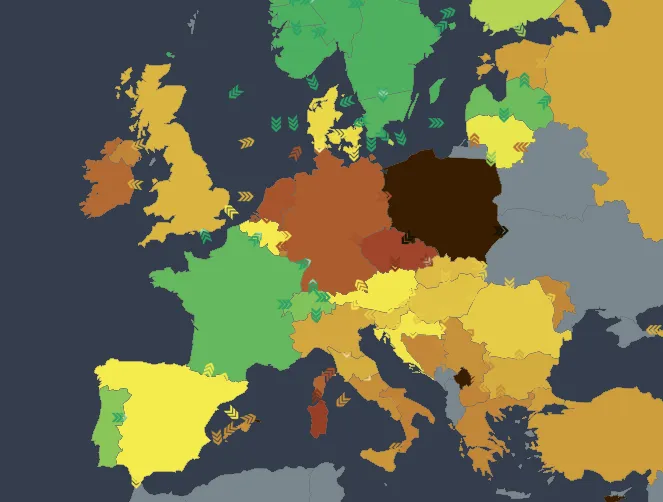

2023年平均碳强度（gCO2eq/kWh）和电力消耗构成（%）。R语言代码如下：

1
2
3
4
5
6
7
8
9
10
11
12
13
14
15
16
17
18
19
20
21
22
23
24
25
26
27
28
29
30
31
32
33
34
35
36
37
38
39
40
41
42
43
44
45
46
47
48
49
50
51
52
53
54
55
56
57
58
59
60
61
62
63
64
65
66
67
68
69
70
71
72
73
74
75
76
77
78
79
# 加载库library(tidyverse)library(gt)library(showtext)showtext_opts(dpi = 300)showtext_auto(enable = TRUE)# 字体font_add_google("Fira Sans Condensed")font_add_google("Oswald", "oswald")# 读取数据power_cie_prepared_tbl <- read_csv("data/power_cie_prepared_tbl.csv")# 创建表格# 注意：虽然碳强度数据是免费提供的，但消耗数据# （水力到电池放电列）需要订阅，因此我创建了一个汇总表格，# 而不是显示前面的数据整理步骤。ciep_gt_tbl <- power_cie_prepared_tbl %>%  gt() %>%  # 应用更宽的颜色范围到碳强度列，以模拟源网站的颜色：  data_color(columns = `CO2 Intensity`,             palette = c("#00A600", "#E6E600", "#E8C32E", "#D69C4E",                         "#Dc863B", "sienna", "sienna4",                         "tomato4", "brown"),             domain = c(0, 900)) %>%  # 应用颜色范围以突出显示低碳发电对降低CO2强度的贡献  data_color(columns = Hydro:Geothermal,             palette = c("#00A600", "chartreuse3", "chartreuse4", "snow") %>% rev(),             domain = c(0, 1),             apply_to = "fill") %>%  # 应用颜色范围以突出显示生物质发电对中等CO2强度的贡献  data_color(columns = Biomass,             palette = c("snow", "#EEC900", "#E8C32E", "#D69C4E"),             domain = c(0, 0.3),             apply_to = "fill") %>%  # 应用颜色范围以突出显示化石燃料对较高CO2强度的贡献  data_color(columns = Gas:Oil,             palette = c("tomato4", "sienna4", "#D69C4E", "#Dc863B", "snow") %>% rev(),             domain = c(0, 1),             apply_to = "fill") %>%  # 为剩余列分配一致的背景颜色  data_color(columns = Unknown:`Battery Discharge`,             palette = c("snow") %>% rev(),             domain = c(0, 1),             apply_to = "fill") %>%  # 为Zone列分配相同的背景  data_color(columns = Zone,             palette = "snow",             apply_to = "fill") %>%  # 添加标题、来源说明和一些样式选项  tab_source_note(md("**表格**: @GrantChalmers | **来源**: api.electricitymap.org | **方法论**: https://www.electricitymaps.com/methodology. 用于计算碳强度的排放因子可在*碳强度和排放因子*选项卡中找到。")) %>%  tab_source_note(source_note = md("某些排放因子基于IPCC 2014默认值，而有些则基于更准确的区域因子。所有区域均可通过Google文档[链接](https://docs.google.com/spreadsheets/d/1ukTAD_oQKZfq-FgLpbLo_bGOv-UPTaoM_WS316xlDcE/edit?usp=sharing)在*碳强度和排放因子*选项卡中公开获取")) %>%  tab_header(md(str_glue("2023年平均**碳强度**（gCO2eq/kWh）和**电力消耗**构成（%）"))) %>%  tab_options(data_row.padding = px(1),              table.font.names = "Fira Sans Condensed",              table.font.size = 12,              table.background.color = 'snow',              heading.background.color = 'antiquewhite',              column_labels.background.color = 'antiquewhite',              source_notes.background.color = 'antiquewhite',              source_notes.font.size = 8) %>%  tab_style_body(style = cell_text(color = "grey60"),                 values = 0) %>%  tab_style(style = cell_text(color = "#A9A9A9", font = "oswald", size = "xx-small", style = "normal"),            locations = cells_source_notes()) %>%  cols_width(2:last_col() ~ px(58)) %>%  cols_align(align = "center", columns = `CO2 Intensity`) %>%  # 转换为百分比  fmt_percent(columns = Hydro:`Battery Discharge`, decimals = 1, drop_trailing_zeros = TRUE) %>%  fmt_number(columns = `CO2 Intensity`, decimals = 0, drop_trailing_zeros = TRUE) %>%  # 对齐小数点以便于阅读  cols_align_decimal(# 排除CO2 Intensity    columns = 3:last_col()) %>%  # 添加边框以改善视觉效果  opt_table_outline()# 渲染表格ciep_gt_tbl

2023年平均碳强度（gCO2eq/kWh）和电力消耗构成（%）

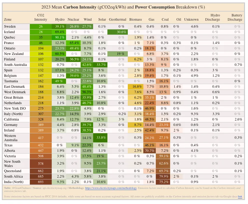
对应的Python代码如下：

1
2
3
4
5
6
7
8
9
10
11
12
13
14
15
16
17
18
19
20
21
22
23
24
25
26
27
28
29
30
31
32
33
34
35
36
37
38
39
40
41
42
43
44
45
46
47
48
49
50
51
52
53
54
55
56
57
58
59
60
61
62
63
64
65
66
67
68
69
70
71
72
73
74
75
76
77
78
79
80
81
82
83
84
85
86
from great_tables import GT, md, html, system_fontsimport pandas as pdpower_cie_prepared_tbl = pd.read_csv("./data/2023_cie_power_cons.csv")# Create a Great Tables objectciep_gt_tbl = GT(data=power_cie_prepared_tbl)# Apply wider color ranges & formattinggt_tbl = ciep_gt_tbl \    .fmt_percent(columns=['Hydro', 'Nuclear', 'Wind', 'Solar', 'Geothermal', 'Biomass', 'Gas',                          'Coal', 'Oil', 'Unknown', 'Hydro Discharge', 'Battery Discharge'],                 decimals=1) \    .fmt_number(columns=['CO2 Intensity'],                 decimals=0) \    .data_color(        columns=['CO2 Intensity'],        palette=[            "#00A600", "#E6E600", "#E8C32E", "#D69C4E", "#Dc863B", "sienna", "sienna4", "tomato4", "brown"],        domain=[0, 900]        ) \    .data_color(        columns=['Hydro', 'Nuclear', 'Wind', 'Solar','Geothermal'],        palette=["#00A600", "chartreuse3", "chartreuse4", "snow"][::-1],        domain=[0, 1]        ) \    .data_color(        columns=['Hydro', 'Geothermal'],        palette=["#00A600", "chartreuse3", "chartreuse4", "snow"][::-1],        domain=[0, 1]        ) \    .data_color(        columns=['Biomass'],        palette=["snow", "#EEC900", "#E8C32E", "#D69C4E"],        domain=[0, 0.3]        ) \    .data_color(        columns=['Gas', 'Coal', 'Oil'],        palette=["tomato4", "sienna4", "#D69C4E", "#Dc863B", "snow"][::-1],        domain=[0, 1]        ) \    .data_color(        columns=['Zone','Unknown', 'Hydro Discharge', 'Battery Discharge'],        palette=["snow", "snow", "snow", 'snow']        ) \    .cols_width(        {'CO2 Intensity': '58px','Hydro': '58px', 'Nuclear': '58px', 'Wind': '58px', 'Solar': '58px',         'Geothermal': '58px', 'Biomass': '58px', 'Gas': '58px', 'Coal': '58px',         'Oil': '58px', 'Unknown': '58px', 'Hydro Discharge': '58px',         'Battery Discharge': '58px'}        ) \    .tab_header(        title=md("2023 Mean **Carbon Intensity** (gCO2eq/kWh) and **Power Consumption** Breakdown (%)")        ) \    .tab_source_note(        md(            '<br><div style="text-align: left;">'            "**Source**: api.electricitymap.org"            " | **Methodology**: https://www.electricitymaps.com/methodology."            " Some emissions factors are based on IPCC 2014 defaults, while some are based on more accurate regional factors."            " <br>All zones are publicly available on the *Carbon intensity and emission factors* tab via Google docs link<br>"            "</div>"            "<br>"            )        ) \    .tab_options(        source_notes_font_size='x-small',        source_notes_padding=3,        table_font_names=system_fonts("humanist"),        data_row_padding='1px',        heading_background_color='antiquewhite',        source_notes_background_color='antiquewhite',        column_labels_background_color='antiquewhite',        table_background_color='snow',        data_row_padding_horizontal=3,        column_labels_padding_horizontal=58        ) \    .cols_align(        align='center'        ) \    .cols_align(        align='left',        columns=['Zone']        )gt_tbl