在前几节中,我们已经建立了完整的统计推断体系:
现在进入一个核心应用:
如何刻画变量之间的关系?
1问题提出
给定数据:
我们希望回答:
当 变化时, 如何变化?
👉 一个自然假设:
2模型解释
👉 核心假设:
3直觉理解
可以理解为:
观测值 = 规律 + 噪声
👉 目标:
找到“最合适”的直线
4最小二乘法(Least Squares)
定义损失函数:
👉 结果:
5Python实现
# file: regression_manual.py
import numpy as np
import matplotlib.pyplot as plt
defmain():
np.random.seed(0)
x = np.linspace(0, 10, 100)
y = 2 + 3*x + np.random.normal(0, 2, 100)
beta1 = np.cov(x, y)[0,1] / np.var(x)
beta0 = np.mean(y) - beta1 * np.mean(x)
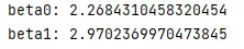
print("beta0:", beta0)
print("beta1:", beta1)
y_pred = beta0 + beta1 * x
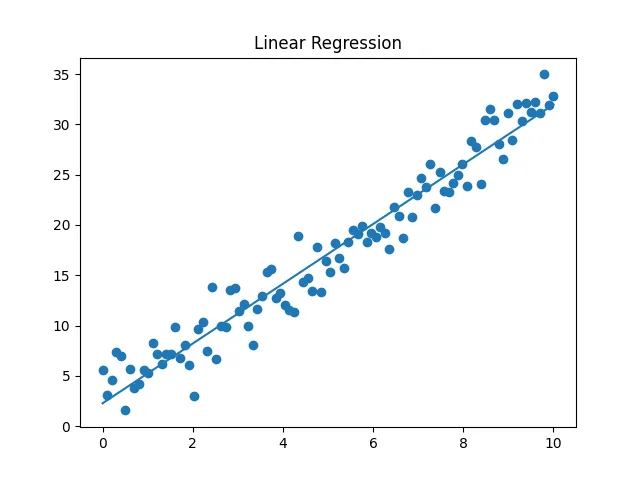
plt.scatter(x, y)
plt.plot(x, y_pred)
plt.title("Linear Regression")
plt.show()
if __name__ == "__main__":
main()
结果解释
6MLE视角
假设:
则:
👉 最大化似然:
等价于:
👉 结论:
最小二乘 = 最大似然估计
7参数分布(推断基础)
在一定条件下:
👉 这使得:
8系数显著性检验
假设:
统计量:
# file: regression_ttest.py
import numpy as np
from scipy import stats
defmain():
np.random.seed(0)
x = np.linspace(0,10,100)
y = 2 + 3*x + np.random.normal(0,2,100)
beta1 = np.cov(x,y)[0,1] / np.var(x)
beta0 = np.mean(y) - beta1*np.mean(x)
y_pred = beta0 + beta1*x
residuals = y - y_pred
s2 = np.sum(residuals**2) / (len(x)-2)
se_beta1 = np.sqrt(s2 / np.sum((x-np.mean(x))**2))
t_stat = beta1 / se_beta1
p_value = 2*(1 - stats.t.cdf(abs(t_stat), df=len(x)-2))
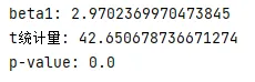
print("beta1:", beta1)
print("t统计量:", t_stat)
print("p-value:", p_value)
if __name__ == "__main__":
main()
结果解释
9拟合优度(R²)
定义:
# file: regression_r2.py
import numpy as np
defmain():
np.random.seed(0)
x = np.linspace(0,10,100)
y = 2 + 3*x + np.random.normal(0,2,100)
beta1 = np.cov(x,y)[0,1] / np.var(x)
beta0 = np.mean(y) - beta1*np.mean(x)
y_pred = beta0 + beta1*x
ss_res = np.sum((y - y_pred)**2)
ss_tot = np.sum((y - np.mean(y))**2)
r2 = 1 - ss_res/ss_tot
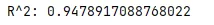
print("R^2:", r2)
if __name__ == "__main__":
main()
执行结果如下: