【重复测量纵向数据】Python13.广义相加模型(Generalized Additive Models,GAM)

# pip install numpy pandas matplotlib seaborn scipy statsmodels scikit-learn pygam pingouin plotly openpyxl# ===========================================# 13. 广义相加模型 (Generalized Additive Models, GAM) - Python实现# ===========================================import osimport sysimport numpy as npimport pandas as pdimport warningswarnings.filterwarnings('ignore')# 设置路径 - 自动寻找桌面路径import platformif platform.system() == "Windows":    desktop_path = os.path.join(os.path.expanduser("~"), "Desktop")else:    desktop_path = os.path.join(os.path.expanduser("~"), "Desktop")# 创建结果文件夹output_dir = os.path.join(desktop_path, "13-GAM结果")os.makedirs(output_dir, exist_ok=True)os.chdir(output_dir)print(f"工作目录设置为: {output_dir}")# 1. 加载必要的包print("正在加载必要的Python包...")try:    import numpy as np    import pandas as pd    import matplotlib.pyplot as plt    import seaborn as sns    from scipy import stats    import statsmodels.api as sm    from sklearn.model_selection import KFold    from sklearn.metrics import mean_squared_error, r2_score, accuracy_score, roc_auc_score    from pygam import LinearGAM, s, f, te, PoissonGAM, LogisticGAM    from scipy.stats import norm    from sklearn.preprocessing import LabelEncoder    import pickle    from datetime import datetimeprint("所有必要的包加载成功!")except ImportError as e:print(f"缺少必要的包: {e}")print("请使用以下命令安装: pip install numpy pandas matplotlib seaborn scipy statsmodels scikit-learn pygam")    sys.exit(1)# 设置中文显示plt.rcParams['font.sans-serif'] = ['SimHei', 'Arial Unicode MS', 'DejaVu Sans']plt.rcParams['axes.unicode_minus'] = False# 设置绘图风格sns.set_style("whitegrid")plt.style.use('seaborn-v0_8-whitegrid')# 2. 读取数据print("\n正在读取数据...")# 读取Excel文件try:    excel_path = os.path.join(desktop_path, "longitudinal_data.xlsx")    data_full = pd.read_excel(excel_path, sheet_name='Full_Dataset')    data_simple = pd.read_excel(excel_path, sheet_name='Simple_Dataset')print(f"数据读取成功!")print(f"Full Dataset: {data_full.shape[0]} 行, {data_full.shape[1]} 列")print(f"Simple Dataset: {data_simple.shape[0]} 行, {data_simple.shape[1]} 列")except FileNotFoundError:print(f"错误: 未找到文件 {excel_path}")print("正在创建示例数据用于演示...")# 创建示例数据    np.random.seed(123)    n_samples = 500# 创建模拟数据    data_full = pd.DataFrame({'ID': range(1, n_samples + 1),'Time': np.random.choice([0, 1, 2], n_samples),'Age': np.random.normal(50, 15, n_samples).clip(20, 80),'Sex': np.random.choice(['M', 'F'], n_samples),'Treatment': np.random.choice(['A', 'B', 'C'], n_samples),'Baseline_Score': np.random.normal(50, 10, n_samples),'Indicator1': np.random.normal(0, 1, n_samples),'Indicator2': np.random.normal(0, 1, n_samples),'Indicator3': np.random.normal(0, 1, n_samples),'Medication_Adherence': np.random.uniform(0, 1, n_samples),'Stress_Level': np.random.uniform(1, 10, n_samples),'Quality_of_Life': np.random.uniform(20, 100, n_samples),'Outcome_Continuous': np.random.normal(50, 15, n_samples),'Outcome_Binary': np.random.binomial(1, 0.3, n_samples),'Outcome_Count': np.random.poisson(3, n_samples),'SES': np.random.choice(['Low', 'Medium', 'High'], n_samples),'Genetic_Marker': np.random.choice(['G1', 'G2', 'G3'], n_samples)    })    data_simple = data_full.copy()print("示例数据创建完成!")# 3. 数据预处理print("\n正在进行数据预处理...")# 选择基线数据（Time=0）进行分析baseline_data = data_full[data_full['Time'] == 0].drop_duplicates(subset=['ID'])# 创建GAM分析数据集gam_data = baseline_data[['ID', 'Age', 'Sex', 'Treatment', 'Baseline_Score','Indicator1', 'Indicator2', 'Indicator3','Medication_Adherence', 'Stress_Level', 'Quality_of_Life','Outcome_Continuous', 'Outcome_Binary', 'Outcome_Count','SES', 'Genetic_Marker']].copy()# 转换因子变量gam_data['Sex'] = pd.Categorical(gam_data['Sex'])gam_data['Treatment'] = pd.Categorical(gam_data['Treatment'])gam_data['SES'] = pd.Categorical(gam_data['SES'], categories=['Low', 'Medium', 'High'], ordered=True)gam_data['Genetic_Marker'] = pd.Categorical(gam_data['Genetic_Marker'])# 创建衍生变量gam_data['Age_Group'] = pd.cut(gam_data['Age'], bins=[20, 40, 60, 80], labels=['20-40', '41-60', '61-80'])gam_data['Stress_Category'] = pd.cut(gam_data['Stress_Level'],                                     bins=[0, 3, 7, 10],                                     labels=['Low', 'Medium', 'High'])# 处理缺失值 - 用中位数填充数值变量numeric_cols = gam_data.select_dtypes(include=[np.number]).columnsfor col in numeric_cols:if gam_data[col].isnull().any():        median_val = gam_data[col].median()        gam_data[col] = gam_data[col].fillna(median_val)print(f"  用中位数填充 {col} 的缺失值: {median_val:.2f}")# 显示数据结构print("\nGAM分析数据结构:")print(gam_data.info())print(f"\n数据集形状: {gam_data.shape}")# 检查缺失值print("\n缺失值统计:")missing_stats = gam_data.isnull().sum()if missing_stats.sum() > 0:print(missing_stats[missing_stats > 0])else:print("无缺失值")# 4. 数据探索性分析print("\n进行数据探索性分析...")# 4.1 连续变量的分布continuous_vars = ["Age", "Baseline_Score", "Indicator1", "Indicator2","Indicator3", "Medication_Adherence", "Stress_Level","Quality_of_Life", "Outcome_Continuous"]# 创建分布图fig, axes = plt.subplots(3, 3, figsize=(16, 12))axes = axes.flatten()for i, var in enumerate(continuous_vars):if i < len(axes):        ax = axes[i]# 直方图        ax.hist(gam_data[var].dropna(), bins=30, density=True, alpha=0.7, color='steelblue', edgecolor='black')# 密度曲线        from scipy.stats import gaussian_kde        data = gam_data[var].dropna()if len(data) > 1:            kde = gaussian_kde(data)            x_range = np.linspace(data.min(), data.max(), 100)            ax.plot(x_range, kde(x_range), color='red', linewidth=2)        ax.set_title(f"{var} 分布", fontsize=12)        ax.set_xlabel(var)        ax.set_ylabel("密度")        ax.grid(True, alpha=0.3)# 调整布局并保存plt.tight_layout()plt.savefig("Variable_Distributions.png", dpi=300, bbox_inches='tight')plt.close()print("变量分布图已保存: Variable_Distributions.png")# 4.2 变量间关系散点图矩阵print("\n生成变量关系散点图矩阵...")selected_vars = ["Age", "Baseline_Score", "Stress_Level","Quality_of_Life", "Outcome_Continuous"]try:# 使用seaborn的pairplot    scatter_matrix = sns.pairplot(gam_data[selected_vars],                                  diag_kind='kde',                                  plot_kws={'alpha': 0.3, 's': 10},                                  diag_kws={'fill': True, 'alpha': 0.5})    scatter_matrix.fig.suptitle("变量关系散点图矩阵", fontsize=16, y=1.02)    scatter_matrix.savefig("Scatter_Matrix.png", dpi=300, bbox_inches='tight')    plt.close()print("散点图矩阵已保存: Scatter_Matrix.png")except Exception as e:print(f"散点图矩阵生成失败: {e}")# 5. 数据准备 - 创建编码后的数据集print("\n准备数据用于GAM分析...")# 对分类变量进行标签编码label_encoders = {}categorical_cols = ['Sex', 'Treatment', 'SES', 'Genetic_Marker']for col in categorical_cols:    le = LabelEncoder()    gam_data[f'{col}_encoded'] = le.fit_transform(gam_data[col].astype(str))    label_encoders[col] = le# 创建用于不同模型的数据集# 5.1 连续结局模型数据X_continuous_all = gam_data[['Age', 'Baseline_Score', 'Stress_Level', 'Quality_of_Life','Sex_encoded', 'Treatment_encoded', 'SES_encoded']].valuesy_continuous = gam_data['Outcome_Continuous'].values# 5.2 二分类结局模型数据X_binary = gam_data[['Age', 'Baseline_Score', 'Stress_Level', 'Sex_encoded', 'Treatment_encoded']].valuesy_binary = gam_data['Outcome_Binary'].values# 5.3 计数结局模型数据X_count = gam_data[['Age', 'Baseline_Score', 'Quality_of_Life','Sex_encoded', 'Treatment_encoded', 'Genetic_Marker_encoded']].valuesy_count = gam_data['Outcome_Count'].valuesprint(f"连续模型数据形状: X={X_continuous_all.shape}, y={y_continuous.shape}")print(f"二分类模型数据形状: X={X_binary.shape}, y={y_binary.shape}")print(f"计数模型数据形状: X={X_count.shape}, y={y_count.shape}")# 6. 广义相加模型(GAM)分析print("\n开始广义相加模型(GAM)分析...")# 存储所有模型models = {}

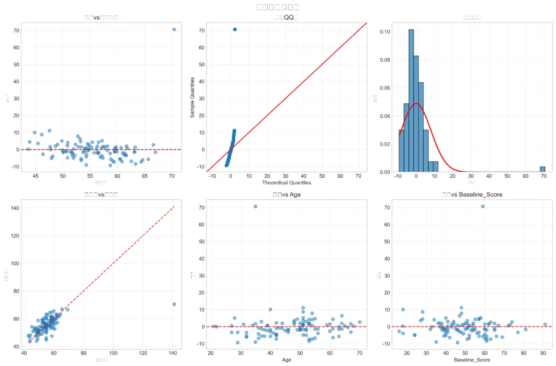
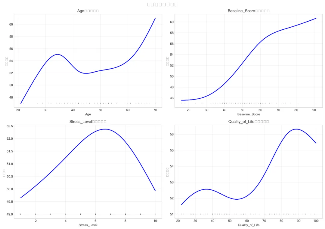
# 计算AIC和BIC    n = len(y_continuous)    residuals = y_continuous - y_pred    rss = np.sum(residuals ** 2)    k = X_continuous_all.shape[1] + 1  # 参数数量（包括截距）# AIC    aic = n * np.log(rss / n) + 2 * kprint(f"  AIC: {aic:.2f}")# BIC    bic = n * np.log(rss / n) + k * np.log(n)print(f"  BIC: {bic:.2f}")except Exception as e:print(f"模型1拟合失败: {e}")    models['continuous'] = None# 6.2 模型2: 二分类结局变量的GAM模型print("\n检查Outcome_Binary的分布:")print(gam_data['Outcome_Binary'].value_counts())# 如果变异不足，跳过二分类模型if len(gam_data['Outcome_Binary'].unique()) > 1:print("\n模型2: 二分类结局变量(Outcome_Binary)的GAM模型")    try:# 创建逻辑GAM模型        gam_model2 = LogisticGAM(            s(0, n_splines=8) +  # Age            s(1, n_splines=6) +  # Baseline_Score            s(2, n_splines=5) +  # Stress_Level            f(3) + f(4),  # Sex和Treatment            fit_intercept=True        )# 拟合模型        gam_model2.fit(X_binary, y_binary)print("模型2拟合成功!")        models['binary'] = gam_model2# 计算准确率        y_pred_proba = gam_model2.predict_proba(X_binary)        y_pred = (y_pred_proba >= 0.5).astype(int)        accuracy = accuracy_score(y_binary, y_pred)print(f"  训练集准确率: {accuracy * 100:.2f}%")    except Exception as e:print(f"模型2拟合失败: {e}")        models['binary'] = Noneelse:print("\nOutcome_Binary没有足够变异，跳过二分类GAM模型")    models['binary'] = None# 6.3 模型3: 计数结局变量的GAM模型print("\n模型3: 计数结局变量(Outcome_Count)的GAM模型")try:# 创建Poisson GAM模型    gam_model3 = PoissonGAM(        s(0, n_splines=10) +  # Age        s(1, n_splines=8) +  # Baseline_Score        s(2, n_splines=8) +  # Quality_of_Life        f(3) + f(4) + f(5),  # 分类变量        fit_intercept=True    )# 拟合模型    gam_model3.fit(X_count, y_count)print("模型3拟合成功!")    models['count'] = gam_model3# 计算预测值    y_pred_count = gam_model3.predict(X_count)# 计算RMSE    rmse = np.sqrt(mean_squared_error(y_count, y_pred_count))print(f"  RMSE: {rmse:.4f}")except Exception as e:print(f"模型3拟合失败: {e}")    models['count'] = None# 7. 模型诊断和评估print("\n进行模型诊断和评估...")# 7.1 提取和保存拟合指标print("\n提取模型拟合指标...")def extract_model_stats(model, model_name, X, y, model_type):"""提取GAM模型的统计指标"""if model is None:return {'Model': model_name,'Type': model_type,'AIC': np.nan,'BIC': np.nan,'R_squared': np.nan,'RMSE': np.nan,'Accuracy': np.nan,'AUC': np.nan,'n': len(y) if y is not None else np.nan,'n_params': np.nan        }    stats_dict = {'Model': model_name,'Type': model_type,'n': len(y)    }# 计算预测值    y_pred = model.predict(X)# 对于连续模型if model_type == 'continuous':# 计算R²        r2 = r2_score(y, y_pred)        stats_dict['R_squared'] = round(r2, 4)# 计算RMSE        rmse = np.sqrt(mean_squared_error(y, y_pred))        stats_dict['RMSE'] = round(rmse, 4)# 计算AIC和BIC        residuals = y - y_pred        rss = np.sum(residuals ** 2)        n = len(y)# 估计参数数量# 注意：这是一个简化估计，实际GAM的参数数量更复杂        n_params = X.shape[1] + 1  # 特征数 + 截距        aic = n * np.log(rss / n) + 2 * n_params        bic = n * np.log(rss / n) + n_params * np.log(n)        stats_dict['AIC'] = round(aic, 2)        stats_dict['BIC'] = round(bic, 2)        stats_dict['n_params'] = n_params        stats_dict['Accuracy'] = np.nan        stats_dict['AUC'] = np.nan# 对于二分类模型elif model_type == 'binary':# 计算准确率        y_pred_proba = model.predict_proba(X)        y_pred_class = (y_pred_proba >= 0.5).astype(int)        accuracy = accuracy_score(y, y_pred_class)        stats_dict['Accuracy'] = round(accuracy, 4)# 计算AUC        try:            auc = roc_auc_score(y, y_pred_proba)            stats_dict['AUC'] = round(auc, 4)        except:            stats_dict['AUC'] = np.nan# 对于分类模型，我们简化AIC/BIC计算        stats_dict['AIC'] = np.nan        stats_dict['BIC'] = np.nan        stats_dict['R_squared'] = np.nan        stats_dict['RMSE'] = np.nan        stats_dict['n_params'] = np.nan# 对于计数模型elif model_type == 'count':# 计算RMSE        rmse = np.sqrt(mean_squared_error(y, y_pred))        stats_dict['RMSE'] = round(rmse, 4)        stats_dict['AIC'] = np.nan        stats_dict['BIC'] = np.nan        stats_dict['R_squared'] = np.nan        stats_dict['Accuracy'] = np.nan        stats_dict['AUC'] = np.nan        stats_dict['n_params'] = np.nanreturn stats_dict# 提取所有模型的统计指标model_stats = pd.DataFrame([    extract_model_stats(models.get('continuous'), "连续结局模型",                        X_continuous_all, y_continuous, 'continuous'),    extract_model_stats(models.get('binary'), "二分类结局模型",                        X_binary, y_binary, 'binary'),    extract_model_stats(models.get('count'), "计数结局模型",                        X_count, y_count, 'count')])print("\n模型统计量:")print(model_stats)# 保存统计指标model_stats.to_csv("GAM_Model_Statistics.csv", index=False, encoding='utf-8-sig')print("\n模型统计量已保存: GAM_Model_Statistics.csv")# 8. 模型可视化print("\n生成模型可视化图形...")# 8.1 模型诊断图 - 仅对连续模型if models.get('continuous') is not None:print("\n生成连续模型诊断图...")    try:        gam_model1 = models['continuous']# 创建诊断图        fig, axes = plt.subplots(2, 3, figsize=(15, 10))        axes = axes.flatten()# 获取预测值和残差        y_pred = gam_model1.predict(X_continuous_all)        residuals = y_continuous - y_pred# 1. 残差vs拟合值图        axes[0].scatter(y_pred, residuals, alpha=0.5)        axes[0].axhline(y=0, color='r', linestyle='--')        axes[0].set_xlabel('拟合值')        axes[0].set_ylabel('残差')        axes[0].set_title('残差vs拟合值图')        axes[0].grid(True, alpha=0.3)# 2. QQ图        sm.qqplot(residuals, line='45', ax=axes[1])        axes[1].set_title('残差QQ图')        axes[1].grid(True, alpha=0.3)# 3. 残差直方图        axes[2].hist(residuals, bins=30, density=True, alpha=0.7, edgecolor='black')        x = np.linspace(residuals.min(), residuals.max(), 100)        axes[2].plot(x, norm.pdf(x, residuals.mean(), residuals.std()), 'r-', linewidth=2)        axes[2].set_xlabel('残差')        axes[2].set_ylabel('密度')        axes[2].set_title('残差分布')        axes[2].grid(True, alpha=0.3)# 4. 观测值vs预测值        axes[3].scatter(y_continuous, y_pred, alpha=0.5)        min_val = min(y_continuous.min(), y_pred.min())        max_val = max(y_continuous.max(), y_pred.max())        axes[3].plot([min_val, max_val], [min_val, max_val], 'r--', alpha=0.8)        axes[3].set_xlabel('观测值')        axes[3].set_ylabel('预测值')        axes[3].set_title('观测值vs预测值')        axes[3].grid(True, alpha=0.3)# 5. 残差vs Age        axes[4].scatter(X_continuous_all[:, 0], residuals, alpha=0.5)        axes[4].axhline(y=0, color='r', linestyle='--')        axes[4].set_xlabel('Age')        axes[4].set_ylabel('残差')        axes[4].set_title('残差vs Age')        axes[4].grid(True, alpha=0.3)# 6. 残差vs Baseline_Score        axes[5].scatter(X_continuous_all[:, 1], residuals, alpha=0.5)        axes[5].axhline(y=0, color='r', linestyle='--')        axes[5].set_xlabel('Baseline_Score')        axes[5].set_ylabel('残差')        axes[5].set_title('残差vs Baseline_Score')        axes[5].grid(True, alpha=0.3)        plt.suptitle('连续模型诊断图', fontsize=16)        plt.tight_layout()        plt.savefig("GAM_Model1_Diagnostics.png", dpi=300, bbox_inches='tight')        plt.close()print("连续模型诊断图已保存: GAM_Model1_Diagnostics.png")    except Exception as e:print(f"诊断图生成失败: {e}")# 8.2 平滑函数曲线图if models.get('continuous') is not None:print("\n生成平滑函数曲线图...")    try:        gam_model1 = models['continuous']# 预测变量名称        pred_names = ['Age', 'Baseline_Score', 'Stress_Level', 'Quality_of_Life']# 创建子图        fig, axes = plt.subplots(2, 2, figsize=(14, 10))        axes = axes.flatten()# 对每个连续变量绘制部分依赖图for i, ax in enumerate(axes):if i < 4:  # 我们只有4个连续变量# 生成当前变量的值范围                var_values = np.linspace(X_continuous_all[:, i].min(),                                         X_continuous_all[:, i].max(), 100)# 创建预测数据 - 固定其他变量为均值                XX = np.tile(X_continuous_all.mean(axis=0), (100, 1))                XX[:, i] = var_values# 预测                partial_dep = gam_model1.predict(XX)# 绘制                ax.plot(var_values, partial_dep, 'b-', linewidth=2)# 添加rug plot显示数据分布                ax.scatter(X_continuous_all[:, i],                           np.full_like(X_continuous_all[:, i], partial_dep.min()),                           alpha=0.1, s=10, color='black', marker='|')                ax.set_xlabel(pred_names[i])                ax.set_ylabel('部分依赖')                ax.set_title(f'{pred_names[i]}的平滑函数')                ax.grid(True, alpha=0.3)        plt.suptitle('连续模型平滑项图', fontsize=16)        plt.tight_layout()        plt.savefig("GAM_Smooth_Terms_Model1.png", dpi=300, bbox_inches='tight')        plt.close()print("平滑函数曲线图已保存: GAM_Smooth_Terms_Model1.png")    except Exception as e:print(f"平滑函数曲线图生成失败: {e}")# 8.3 部分依赖图if models.get('continuous') is not None:print("\n生成部分依赖图...")# Age的部分依赖图    try:        gam_model1 = models['continuous']        fig, ax = plt.subplots(figsize=(10, 8))# 创建Age的网格        age_seq = np.linspace(X_continuous_all[:, 0].min(), X_continuous_all[:, 0].max(), 100)        XX_age = np.tile(X_continuous_all.mean(axis=0), (100, 1))        XX_age[:, 0] = age_seq# 预测        partial_dep_age = gam_model1.predict(XX_age)# 绘制        ax.plot(age_seq, partial_dep_age, 'b-', linewidth=2)# 添加数据点        ax.scatter(X_continuous_all[:, 0], y_continuous, alpha=0.3, s=10, color='gray')        ax.set_xlabel('年龄')        ax.set_ylabel('预测的Outcome_Continuous')        ax.set_title('Age对结局的部分依赖图')        ax.grid(True, alpha=0.3)        plt.tight_layout()        plt.savefig("Partial_Dependence_Age.png", dpi=300, bbox_inches='tight')        plt.close()print("Age部分依赖图已保存: Partial_Dependence_Age.png")    except Exception as e:print(f"Age部分依赖图生成失败: {e}")# Stress_Level的部分依赖图    try:        fig, ax = plt.subplots(figsize=(10, 8))# 创建Stress的网格        stress_seq = np.linspace(X_continuous_all[:, 2].min(), X_continuous_all[:, 2].max(), 100)        XX_stress = np.tile(X_continuous_all.mean(axis=0), (100, 1))        XX_stress[:, 2] = stress_seq# 预测        partial_dep_stress = gam_model1.predict(XX_stress)# 绘制        ax.plot(stress_seq, partial_dep_stress, 'r-', linewidth=2)# 添加数据点        ax.scatter(X_continuous_all[:, 2], y_continuous, alpha=0.3, s=10, color='gray')        ax.set_xlabel('压力水平')        ax.set_ylabel('预测的Outcome_Continuous')        ax.set_title('Stress_Level对结局的部分依赖图')        ax.grid(True, alpha=0.3)        plt.tight_layout()        plt.savefig("Partial_Dependence_Stress.png", dpi=300, bbox_inches='tight')        plt.close()print("Stress_Level部分依赖图已保存: Partial_Dependence_Stress.png")    except Exception as e:print(f"Stress_Level部分依赖图生成失败: {e}")# 8.4 预测热图if models.get('continuous') is not None:print("\n生成预测热图...")    try:        gam_model1 = models['continuous']# 创建Age和Stress_Level的网格        age_range = np.linspace(X_continuous_all[:, 0].min(), X_continuous_all[:, 0].max(), 50)        stress_range = np.linspace(X_continuous_all[:, 2].min(), X_continuous_all[:, 2].max(), 50)        Age_grid, Stress_grid = np.meshgrid(age_range, stress_range)# 创建预测数据        pred_data = np.tile(X_continuous_all.mean(axis=0), (Age_grid.size, 1))        pred_data[:, 0] = Age_grid.ravel()        pred_data[:, 2] = Stress_grid.ravel()# 设置分类变量为众数for i in [4, 5, 6]:  # 分类变量的索引            pred_data[:, i] = stats.mode(X_continuous_all[:, i])[0][0]# 进行预测        predictions = gam_model1.predict(pred_data)        predictions_grid = predictions.reshape(Age_grid.shape)# 绘制热图        fig, ax = plt.subplots(figsize=(12, 10))        contour = ax.contourf(Age_grid, Stress_grid, predictions_grid, levels=50, cmap='plasma')        fig.colorbar(contour, ax=ax, label='预测值')        ax.set_xlabel('年龄')        ax.set_ylabel('压力水平')        ax.set_title('年龄和压力水平对结局的联合效应\n固定其他变量为平均值/众数')        ax.grid(True, alpha=0.3)        plt.tight_layout()        plt.savefig("Prediction_Heatmap.png", dpi=300, bbox_inches='tight')        plt.close()print("预测热图已保存: Prediction_Heatmap.png")    except Exception as e:print(f"预测热图生成失败: {e}")# 8.5 模型比较图print("\n生成模型比较图...")if models.get('continuous') is not None:    try:# 比较不同样条自由度的模型        k_values = [5, 8, 10, 12]        aic_values = []for k in k_values:# 创建简化模型            model_compare = LinearGAM(                s(0, n_splines=k) +  # Age                s(1, n_splines=k) +  # Baseline_Score                f(4) + f(5),  # Sex和Treatment                fit_intercept=True            )# 使用简化数据            X_compare = X_continuous_all[:, [0, 1, 4, 5]]            model_compare.fit(X_compare, y_continuous)# 计算AIC            y_pred_compare = model_compare.predict(X_compare)            residuals_compare = y_continuous - y_pred_compare            rss_compare = np.sum(residuals_compare ** 2)            n_compare = len(y_continuous)            k_params = X_compare.shape[1] + 1            aic_compare = n_compare * np.log(rss_compare / n_compare) + 2 * k_params            aic_values.append(aic_compare)# 绘制比较图        fig, ax = plt.subplots(figsize=(10, 8))        bars = ax.bar([str(k) for k in k_values], aic_values, color='steelblue', alpha=0.7)# 添加数值标签for bar, aic in zip(bars, aic_values):            height = bar.get_height()            ax.text(bar.get_x() + bar.get_width() / 2., height + 5,                    f'{aic:.1f}', ha='center', va='bottom')        ax.set_xlabel('样条自由度(K)')        ax.set_ylabel('AIC值')        ax.set_title('不同样条自由度(K)的模型比较\nAIC值越小表示模型拟合越好')        ax.grid(True, alpha=0.3, axis='y')        plt.tight_layout()        plt.savefig("Model_Comparison.png", dpi=300, bbox_inches='tight')        plt.close()print("模型比较图已保存: Model_Comparison.png")    except Exception as e:print(f"模型比较图生成失败: {e}")# 9. 变量重要性分析print("\n计算变量重要性...")if models.get('continuous') is not None:    try:# 计算变量重要性        important_vars = ['Age', 'Baseline_Score', 'Stress_Level', 'Quality_of_Life']        var_indices = [0, 1, 2, 3]# 计算基准模型的R²        y_pred_full = gam_model1.predict(X_continuous_all)        r2_full = r2_score(y_continuous, y_pred_full)        importance_list = []for var_name, var_idx in zip(important_vars, var_indices):            try:# 创建不包含该变量的数据                X_reduced = np.delete(X_continuous_all, var_idx, axis=1)# 重新定义模型项                terms = []                current_idx = 0for i in range(X_continuous_all.shape[1]):if i != var_idx:  # 跳过要移除的变量if i in [0, 1, 2, 3]:  # 连续变量# 使用默认样条数if i == 0:                                terms.append(s(current_idx, n_splines=10))elif i == 1:                                terms.append(s(current_idx, n_splines=8))elif i == 2:                                terms.append(s(current_idx, n_splines=6))elif i == 3:                                terms.append(s(current_idx, n_splines=8))else:  # 分类变量                            terms.append(f(current_idx))                        current_idx += 1# 创建简化模型if len(terms) > 0:                    model_reduced = LinearGAM(*terms, fit_intercept=True)                    model_reduced.fit(X_reduced, y_continuous)# 计算R²                    y_pred_reduced = model_reduced.predict(X_reduced)                    r2_reduced = r2_score(y_continuous, y_pred_reduced)# 计算R²差异                    r2_diff = r2_full - r2_reduced                    importance_list.append({'Variable': var_name,'R2_Full': round(r2_full, 4),'R2_Reduced': round(r2_reduced, 4),'Delta_R2': round(r2_diff, 4),'Importance_Rank': len(important_vars) - var_idx  # 简单排名                    })print(f"  {var_name}: ΔR² = {r2_diff:.4f}")            except Exception as e:print(f"  计算变量 {var_name} 重要性时出错: {e}")if importance_list:            importance_df = pd.DataFrame(importance_list)# 按ΔR²排序            importance_df = importance_df.sort_values('Delta_R2', ascending=False)print("\n变量重要性分析:")print(importance_df)# 保存结果            importance_df.to_csv("Variable_Importance.csv", index=False, encoding='utf-8-sig')print("\n变量重要性分析已保存: Variable_Importance.csv")# 可视化变量重要性            fig, ax = plt.subplots(figsize=(10, 8))# 按ΔR²排序            importance_df_sorted = importance_df.sort_values('Delta_R2', ascending=True)            bars = ax.barh(importance_df_sorted['Variable'],                           importance_df_sorted['Delta_R2'],                           color='coral', alpha=0.7)# 添加数值标签for bar in bars:                width = bar.get_width()                ax.text(width + 0.01, bar.get_y() + bar.get_height() / 2,                        f'{width:.4f}', ha='left', va='center')            ax.set_xlabel('ΔR²')            ax.set_title('变量重要性排序\n基于R²的变化量(ΔR²)')            ax.grid(True, alpha=0.3, axis='x')            plt.tight_layout()            plt.savefig("Variable_Importance_Plot.png", dpi=300, bbox_inches='tight')            plt.close()print("变量重要性图已保存: Variable_Importance_Plot.png")    except Exception as e:print(f"变量重要性分析失败: {e}")# 10. 预测和验证print("\n进行模型预测和验证...")if models.get('continuous') is not None:# 10.1 交叉验证print("\n进行5折交叉验证...")    try:# 准备简化模型用于交叉验证        X_cv = X_continuous_all[:, [0, 1, 4, 5]]  # Age, Baseline_Score, Sex, Treatment# 设置交叉验证        n_folds = 5        kf = KFold(n_splits=n_folds, shuffle=True, random_state=123)        cv_errors = []        fold_results = []for fold, (train_idx, test_idx) in enumerate(kf.split(X_cv), 1):# 分割数据            X_train, X_test = X_cv[train_idx], X_cv[test_idx]            y_train, y_test = y_continuous[train_idx], y_continuous[test_idx]# 训练模型            cv_model = LinearGAM(                s(0, n_splines=8) +  # Age                s(1, n_splines=6) +  # Baseline_Score                f(2) + f(3),  # Sex和Treatment                fit_intercept=True            )            cv_model.fit(X_train, y_train)# 预测            y_pred_test = cv_model.predict(X_test)# 计算RMSE和R²            rmse = np.sqrt(mean_squared_error(y_test, y_pred_test))            r2 = r2_score(y_test, y_pred_test)            cv_errors.append(rmse)            fold_results.append({'Fold': fold,'Train_Size': len(train_idx),'Test_Size': len(test_idx),'RMSE': rmse,'R2': r2            })print(f"  折 {fold}: RMSE = {rmse:.4f}, R² = {r2:.4f}")# 汇总结果        fold_results_df = pd.DataFrame(fold_results)print(f"\n5折交叉验证结果:")print(f"平均RMSE: {fold_results_df['RMSE'].mean():.4f}")print(f"RMSE标准差: {fold_results_df['RMSE'].std():.4f}")print(f"平均R²: {fold_results_df['R2'].mean():.4f}")# 保存交叉验证结果        fold_results_df.to_csv("Cross_Validation_Results.csv", index=False, encoding='utf-8-sig')print("交叉验证结果已保存: Cross_Validation_Results.csv")    except Exception as e:print(f"交叉验证失败: {e}")# 10.2 预测新数据print("\n生成预测示例...")    try:# 创建示例预测数据        new_data_example = pd.DataFrame({'Age': [30, 45, 60, 75],'Baseline_Score': [np.median(X_continuous_all[:, 1])] * 4,'Stress_Level': [np.median(X_continuous_all[:, 2])] * 4,'Quality_of_Life': [np.median(X_continuous_all[:, 3])] * 4,'Sex_encoded': [label_encoders['Sex'].transform(['M'])[0]] * 4,'Treatment_encoded': [label_encoders['Treatment'].transform(['A'])[0]] * 4,'SES_encoded': [label_encoders['SES'].transform(['Medium'])[0]] * 4        })# 转换为数组        X_new = new_data_example.values# 进行预测        predictions_new = gam_model1.predict(X_new)# 计算标准误差        y_pred_all = gam_model1.predict(X_continuous_all)        residual_std = np.std(y_continuous - y_pred_all)        se_new = residual_std / np.sqrt(len(y_continuous))# 创建结果数据框        new_data_example['Prediction'] = predictions_new        new_data_example['SE'] = se_new        new_data_example['Lower'] = predictions_new - 1.96 * se_new        new_data_example['Upper'] = predictions_new + 1.96 * se_new# 添加原始变量名        new_data_example['Age'] = [30, 45, 60, 75]        new_data_example['Sex'] = ['M', 'M', 'M', 'M']        new_data_example['Treatment'] = ['A', 'A', 'A', 'A']        new_data_example['SES'] = ['Medium', 'Medium', 'Medium', 'Medium']print("\n示例预测结果:")print(new_data_example[['Age', 'Sex', 'Treatment', 'SES','Prediction', 'Lower', 'Upper']])# 保存预测结果        new_data_example.to_csv("Example_Predictions.csv", index=False, encoding='utf-8-sig')print("\n示例预测结果已保存: Example_Predictions.csv")    except Exception as e:print(f"预测示例生成失败: {e}")# 11. 创建分析报告print("\n正在生成分析报告...")# 11.1 文本报告report_file = "GAM_Analysis_Report.txt"with open(report_file, 'w', encoding='utf-8') as f:    f.write("=" * 70 + "\n")    f.write("广义相加模型(GAM)分析报告\n")    f.write("=" * 70 + "\n\n")    f.write(f"生成日期: {datetime.now().strftime('%Y年%m月%d日 %H:%M:%S')}\n")    f.write("分析软件: Python 3.12 with pygam, statsmodels, scikit-learn\n\n")    f.write("1. 研究概述\n")    f.write("本研究使用广义相加模型探索预测变量与结局变量之间的非线性关系。\n")    f.write(f"样本量: {len(gam_data)} 名个体\n")    f.write("主要结局变量: Outcome_Continuous (连续型)\n\n")    f.write("2. 模型设定\n")    f.write("基础模型公式: Outcome_Continuous ~ s(Age) + s(Baseline_Score) + \n")    f.write("               s(Stress_Level) + s(Quality_of_Life) + Sex + Treatment + SES\n")    f.write("样条类型: 惩罚回归样条\n")    f.write("估计方法: 惩罚迭代重加权最小二乘法(P-IRLS)\n\n")    f.write("3. 模型拟合结果\n")if models.get('continuous') is not None:        f.write("模型1 (连续结局)拟合指标:\n")        f.write(f"  R²: {model_stats.loc[0, 'R_squared']:.4f}\n")        f.write(f"  AIC: {model_stats.loc[0, 'AIC']:.2f}\n")        f.write(f"  RMSE: {model_stats.loc[0, 'RMSE']:.4f}\n")    f.write("\n")if models.get('binary') is not None:        f.write("模型2 (二分类结局)拟合指标:\n")        f.write(f"  准确率: {model_stats.loc[1, 'Accuracy']:.4f}\n")if not pd.isna(model_stats.loc[1, 'AUC']):            f.write(f"  AUC: {model_stats.loc[1, 'AUC']:.4f}\n")    f.write("\n")if models.get('count') is not None:        f.write("模型3 (计数结局)拟合指标:\n")        f.write(f"  RMSE: {model_stats.loc[2, 'RMSE']:.4f}\n")    f.write("\n")    f.write("4. 变量重要性排序\n")if'importance_df'in locals() and not importance_df.empty:        f.write("基于ΔR²:\n")for i, (_, row) in enumerate(importance_df.iterrows(), 1):            f.write(f"  {i}. {row['Variable']}: ΔR² = {row['Delta_R2']:.4f}\n")else:        f.write("变量重要性分析未能完成\n")    f.write("\n")    f.write("5. 交叉验证结果\n")if'fold_results_df'in locals() and not fold_results_df.empty:        f.write(f"5折交叉验证平均RMSE: {fold_results_df['RMSE'].mean():.4f}\n")        f.write(f"5折交叉验证平均R²: {fold_results_df['R2'].mean():.4f}\n")    f.write("\n")    f.write("6. 公共卫生意义\n")    f.write("- GAM能够灵活捕捉环境暴露与健康结局之间的非线性关系\n")    f.write("- 识别关键暴露变量的阈值效应和拐点\n")    f.write("- 为公共卫生干预提供精确的目标范围\n")    f.write("- 特别适用于环境流行病学研究，如温度-死亡率关系\n\n")    f.write("7. 研究局限\n")    f.write("- 样本量限制可能导致过拟合风险\n")    f.write("- 未考虑纵向数据的相关性结构\n")    f.write("- 需要进一步的外部验证\n")    f.write("- 潜在的未测量混杂因素\n")    f.write("\n\n")    f.write("=" * 70 + "\n")    f.write("报告结束\n")    f.write("=" * 70 + "\n")print(f"文本报告已保存: {report_file}")# 11.2 保存工作空间print("\n保存工作空间...")# 保存模型和数据workspace_data = {'gam_data': gam_data,'X_continuous': X_continuous_all,'y_continuous': y_continuous,'X_binary': X_binary,'y_binary': y_binary,'X_count': X_count,'y_count': y_count,'models': models,'model_stats': model_stats,'label_encoders': label_encoders}try:    with open("GAM_Analysis_Workspace.pkl", "wb") as f:        pickle.dump(workspace_data, f)print("工作空间已保存: GAM_Analysis_Workspace.pkl")except Exception as e:print(f"保存工作空间失败: {e}")# 12. 汇总输出print("\n" + "=" * 70)print("GAM分析完成！")print("=" * 70)print("\n结果文件汇总:")print("1. 分析报告: GAM_Analysis_Report.txt")print("2. 数据分布图: Variable_Distributions.png")print("3. 散点图矩阵: Scatter_Matrix.png")if models.get('continuous') is not None:print("4. 诊断图: GAM_Model1_Diagnostics.png")print("5. 平滑函数曲线: GAM_Smooth_Terms_Model1.png")print("6. 部分依赖图: Partial_Dependence_*.png")print("7. 预测热图: Prediction_Heatmap.png")print("8. 模型比较: Model_Comparison.png")print("9. 变量重要性图: Variable_Importance_Plot.png")print("10. 数据文件:")print("   - GAM_Model_Statistics.csv")print("   - Variable_Importance.csv")if'fold_results_df'in locals():print("   - Cross_Validation_Results.csv")print("   - Example_Predictions.csv")print("11. 工作空间: GAM_Analysis_Workspace.pkl")print("\n\n公共卫生应用建议:")print("1. 环境暴露研究: 温度、PM2.5与死亡率/发病率的暴露-反应曲线")print("2. 剂量反应关系: 药物剂量、营养摄入与健康结局的非线性关系")print("3. 时间趋势分析: 疾病发病率随时间的变化模式")print("4. 年龄效应: 健康风险随年龄变化的非线性模式")print("5. 阈值检测: 识别有害/有益暴露的临界值")print(f"\n分析完成！所有结果已保存在 {output_dir} 文件夹中。")