《15节课Python绘图从入门到精通》6——百分比堆积条形图与复合饼图

前置数据准备

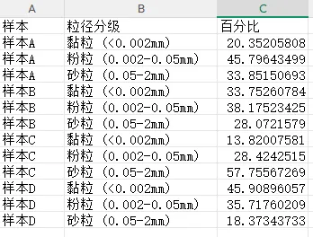
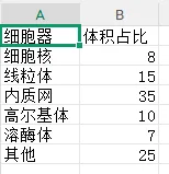
为保证所有程序可直接运行，先运行以下代码生成两组实验数据：土壤粒径分级多组样本数据、细胞器体积占比数据。

import pandas as pdimport numpy as npnp.random.seed(2024)# 模拟四个土壤样本，每个样本三个粒径级别（黏粒、粉粒、砂粒）的百分比samples = ['样本A', '样本B', '样本C', '样本D']fractions = ['黏粒 (<0.002mm)', '粉粒 (0.002-0.05mm)', '砂粒 (0.05-2mm)']data_soil = []for i, sample in enumerate(samples):# 生成不同组成的百分比（和为100%）if i == 0:        clay, silt, sand = 20, 45, 35elif i == 1:        clay, silt, sand = 35, 40, 25elif i == 2:        clay, silt, sand = 15, 30, 55else:        clay, silt, sand = 45, 35, 20# 添加少量随机扰动    clay += np.random.uniform(-2, 2)    silt += np.random.uniform(-2, 2)    sand = 100 - clay - silt  # 确保总和为100    data_soil.append([sample, fractions[0], clay])    data_soil.append([sample, fractions[1], silt])    data_soil.append([sample, fractions[2], sand])df_soil = pd.DataFrame(data_soil, columns=['样本', '粒径分级', '百分比'])df_soil.to_csv('土壤粒径数据.csv', index=False, encoding='utf-8-sig')organelles = ['细胞核', '线粒体', '内质网', '高尔基体', '溶酶体', '其他']volumes = [8, 15, 35, 10, 7, 25]  # 总体积占比（%）df_organelle = pd.DataFrame({'细胞器': organelles, '体积占比': volumes})df_organelle.to_csv('细胞器体积数据.csv', index=False, encoding='utf-8-sig')# 一级分类：主要生物类群level1 = ['细菌', '真菌', '病毒', '原生生物']level1_pct = [45, 30, 15, 10]# 二级分类：各一级分类下的细分bacteria_sub = ['变形菌门', '厚壁菌门', '放线菌门', '拟杆菌门']bacteria_pct = [40, 30, 20, 10]fungi_sub = ['子囊菌门', '担子菌门', '接合菌门']fungi_pct = [50, 35, 15]virus_sub = ['dsDNA病毒', 'ssRNA病毒', 'dsRNA病毒']virus_pct = [60, 30, 10]protozoa_sub = ['鞭毛虫', '阿米巴', '纤毛虫']protozoa_pct = [50, 30, 20]# 构建数据框data_pie = []for sub, pct in zip(bacteria_sub, bacteria_pct):    data_pie.append(['细菌', sub, pct])for sub, pct in zip(fungi_sub, fungi_pct):    data_pie.append(['真菌', sub, pct])for sub, pct in zip(virus_sub, virus_pct):    data_pie.append(['病毒', sub, pct])for sub, pct in zip(protozoa_sub, protozoa_pct):    data_pie.append(['原生生物', sub, pct])df_pie = pd.DataFrame(data_pie, columns=['一级分类', '二级分类', '百分比'])df_pie.to_csv('微生物层级数据.csv', index=False, encoding='utf-8-sig')print("数据生成完成：")print("- 土壤粒径数据.csv（6.1节用）")print("- 细胞器体积数据.csv（6.2节用）")print("- 微生物层级数据.csv（6.3节用）")

执行结果如下：

土壤粒径数据

细胞器体积数据

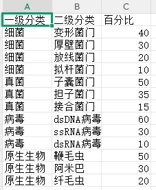
微生物层级数据

实操任务1：绘制多组样本的百分比堆积条形图，标注百分比数值

本任务从基础的百分比堆积条形图入手，逐步进阶到数值标注、自定义配色、排序优化及多分类对比。

基础版：多组样本百分比堆积条形图

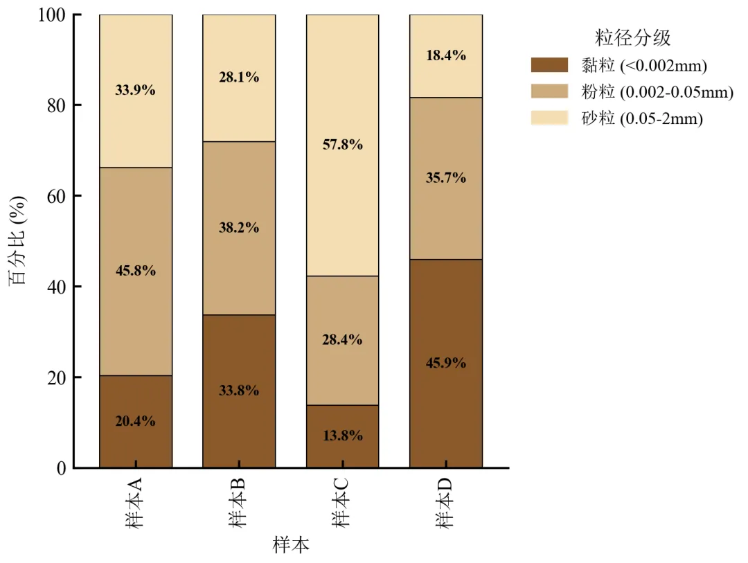
程序读取土壤粒径数据，将数据透视为宽表格式，绘制百分比堆积条形图。

import pandas as pdimport numpy as npimport matplotlib.pyplot as plt# 学术样式设置defset_academic_style():    plt.rcParams['font.family'] = ['Times New Roman', 'SimSun']    plt.rcParams['font.size'] = 9    plt.rcParams['axes.unicode_minus'] = False    plt.rcParams['axes.linewidth'] = 1.0    plt.rcParams['xtick.major.width'] = 1.0    plt.rcParams['ytick.major.width'] = 1.0    plt.rcParams['xtick.major.size'] = 3.5    plt.rcParams['ytick.major.size'] = 3.5    plt.rcParams['xtick.direction'] = 'in'    plt.rcParams['ytick.direction'] = 'in'    plt.rcParams['legend.frameon'] = False    plt.rcParams['pdf.fonttype'] = 42    plt.rcParams['savefig.dpi'] = 300set_academic_style()# 读取数据df = pd.read_csv('土壤粒径数据.csv')# 透视表：行为样本，列为粒径分级，值为百分比df_pivot = df.pivot(index='样本', columns='粒径分级', values='百分比')# 确保列顺序（黏粒、粉粒、砂粒）order = ['黏粒 (<0.002mm)', '粉粒 (0.002-0.05mm)', '砂粒 (0.05-2mm)']df_pivot = df_pivot[order]# 绘制百分比堆积条形图fig, ax = plt.subplots(figsize=(5.0, 3.8))# 使用自定义颜色（土壤学常用色）colors = ['#8B5A2B', '#CDAA7D', '#F5DEB3']  # 深棕、浅棕、米黄df_pivot.plot(kind='bar', stacked=True, ax=ax, color=colors, width=0.7, edgecolor='black', linewidth=0.5)ax.set_xlabel('样本')ax.set_ylabel('百分比 (%)')ax.set_ylim(0, 100)ax.legend(title='粒径分级', bbox_to_anchor=(1.02, 1), loc='upper left', fontsize=8, title_fontsize=9)# 去除上、右 spinesax.spines['top'].set_visible(False)ax.spines['right'].set_visible(False)plt.tight_layout()plt.show()fig.savefig('百分比堆积条形图_基础.pdf', bbox_inches='tight', pad_inches=0.05)fig.savefig('百分比堆积条形图_基础.png', bbox_inches='tight', pad_inches=0.05)

执行结果分析：

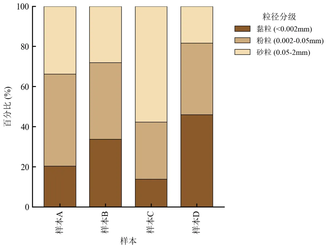
每个样本的条形总高度为100%，直观对比各样本中黏粒、粉粒、砂粒的占比差异。

样本D黏粒比例最高（约45%），样本C砂粒比例最高（约55%），反映土壤质地差异。

图例移至右侧避免遮挡，学术配色符合土壤学常见习惯。

进阶1：在堆积条形图上标注百分比数值

在每段堆积条内部或上方标注具体百分比值，便于精确读取。

import pandas as pdimport numpy as npimport matplotlib.pyplot as pltdefset_academic_style():    plt.rcParams['font.family'] = ['Times New Roman', 'SimSun']    plt.rcParams['font.size'] = 9    plt.rcParams['axes.unicode_minus'] = False    plt.rcParams['axes.linewidth'] = 1.0    plt.rcParams['xtick.major.width'] = 1.0    plt.rcParams['ytick.major.width'] = 1.0    plt.rcParams['xtick.major.size'] = 3.5    plt.rcParams['ytick.major.size'] = 3.5    plt.rcParams['xtick.direction'] = 'in'    plt.rcParams['ytick.direction'] = 'in'    plt.rcParams['legend.frameon'] = False    plt.rcParams['pdf.fonttype'] = 42    plt.rcParams['savefig.dpi'] = 300set_academic_style()df = pd.read_csv('土壤粒径数据.csv')df_pivot = df.pivot(index='样本', columns='粒径分级', values='百分比')order = ['黏粒 (<0.002mm)', '粉粒 (0.002-0.05mm)', '砂粒 (0.05-2mm)']df_pivot = df_pivot[order]colors = ['#8B5A2B', '#CDAA7D', '#F5DEB3']fig, ax = plt.subplots(figsize=(5.0, 3.8))bars = df_pivot.plot(kind='bar', stacked=True, ax=ax, color=colors, width=0.7,                      edgecolor='black', linewidth=0.5, legend=False)# 手动添加图例（控制顺序）handles = [plt.Rectangle((0,0),1,1, color=colors[i]) for i in range(3)]ax.legend(handles, order, title='粒径分级', bbox_to_anchor=(1.02, 1), loc='upper left',           fontsize=8, title_fontsize=9)# 标注百分比（仅当百分比>5%时标注，避免重叠）for i, sample in enumerate(df_pivot.index):    cumulative = 0for j, fraction in enumerate(order):        value = df_pivot.loc[sample, fraction]if value > 5:  # 大于5%才标注            ax.text(i, cumulative + value/2, f'{value:.1f}%',                     ha='center', va='center', fontsize=7, color='black', fontweight='bold')        cumulative += valueax.set_xlabel('样本')ax.set_ylabel('百分比 (%)')ax.set_ylim(0, 100)ax.spines['top'].set_visible(False)ax.spines['right'].set_visible(False)plt.tight_layout()plt.show()fig.savefig('百分比堆积条形图_数值标注.pdf', bbox_inches='tight', pad_inches=0.05)fig.savefig('百分比堆积条形图_数值标注.png', bbox_inches='tight', pad_inches=0.05)

执行结果分析：

每段堆积条中心标注百分比值，清晰显示各粒径级具体占比。

为避免文字重叠，仅标注>5%的段落；对于极小比例可标注在外侧或用引线。

数值标注使读者无需对照坐标轴即可获取精确数据，符合学术严谨性要求。

进阶2：自定义色板与主题（ColorBrewer配色 + 简洁主题）

使用专业配色库palettable或ColorBrewer配色方案，并去除图表冗余元素。

import pandas as pdimport matplotlib.pyplot as pltimport matplotlib.patches as mpatchesdefset_academic_style():    plt.rcParams['font.family'] = ['Times New Roman', 'SimSun']    plt.rcParams['font.size'] = 9    plt.rcParams['axes.unicode_minus'] = False    plt.rcParams['axes.linewidth'] = 1.0    plt.rcParams['xtick.major.width'] = 1.0    plt.rcParams['ytick.major.width'] = 1.0    plt.rcParams['xtick.major.size'] = 3.5    plt.rcParams['ytick.major.size'] = 3.5    plt.rcParams['xtick.direction'] = 'in'    plt.rcParams['ytick.direction'] = 'in'    plt.rcParams['legend.frameon'] = False    plt.rcParams['pdf.fonttype'] = 42    plt.rcParams['savefig.dpi'] = 300set_academic_style()df = pd.read_csv('土壤粒径数据.csv')df_pivot = df.pivot(index='样本', columns='粒径分级', values='百分比')order = ['黏粒 (<0.002mm)', '粉粒 (0.002-0.05mm)', '砂粒 (0.05-2mm)']df_pivot = df_pivot[order]# 使用Tableau 10色板的前三色（土壤色系替代方案）colors = ['#4E79A7', '#F28E2B', '#E15759']  # 蓝、橙、红（对比鲜明）fig, ax = plt.subplots(figsize=(5.0, 3.5))df_pivot.plot(kind='bar', stacked=True, ax=ax, color=colors, width=0.7,               edgecolor='white', linewidth=0.8, legend=False)# 自定义图例（横向排列在顶部）handles = [mpatches.Patch(color=colors[i], label=order[i]) for i in range(3)]ax.legend(handles=handles, loc='upper center', bbox_to_anchor=(0.5, 1.12),           ncol=3, fontsize=8, frameon=False)ax.set_xlabel('样本')ax.set_ylabel('百分比 (%)')ax.set_ylim(0, 100)# 完全去除所有spinesfor spine in ax.spines.values():    spine.set_visible(False)# 仅保留左侧刻度线ax.tick_params(left=True, bottom=False)plt.tight_layout()plt.show()fig.savefig('百分比堆积条形图_简洁主题.pdf', bbox_inches='tight', pad_inches=0.05)fig.savefig('百分比堆积条形图_简洁主题.png', bbox_inches='tight', pad_inches=0.05)

执行结果分析：

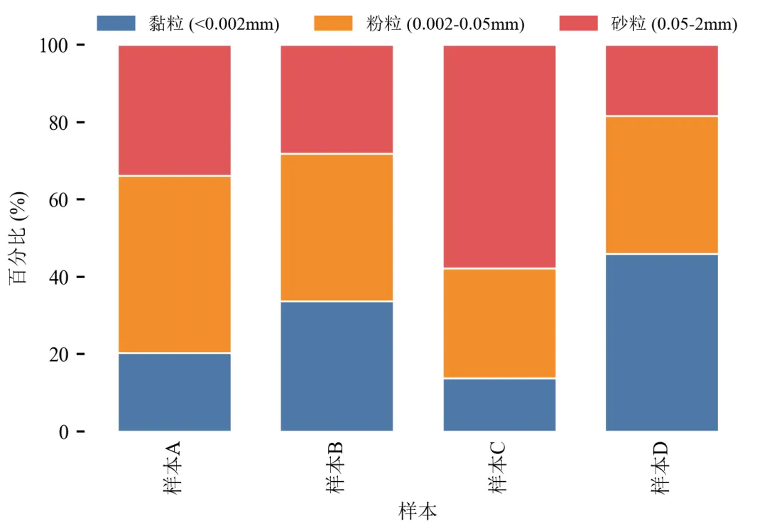
去除顶部和右侧spines，甚至去除所有边框，仅保留左侧坐标轴，画面极简。

图例横向置于图上方，节省横向空间，适合单栏排版。

Tableau配色鲜艳且色盲友好，适合多分类对比。

进阶3：按某组分含量排序样本

将样本按某一组分（如黏粒含量）降序排列，突出该组分的变化趋势。

import pandas as pdimport matplotlib.pyplot as pltdefset_academic_style():    plt.rcParams['font.family'] = ['Times New Roman', 'SimSun']    plt.rcParams['font.size'] = 9    plt.rcParams['axes.unicode_minus'] = False    plt.rcParams['axes.linewidth'] = 1.0    plt.rcParams['xtick.major.width'] = 1.0    plt.rcParams['ytick.major.width'] = 1.0    plt.rcParams['xtick.major.size'] = 3.5    plt.rcParams['ytick.major.size'] = 3.5    plt.rcParams['xtick.direction'] = 'in'    plt.rcParams['ytick.direction'] = 'in'    plt.rcParams['legend.frameon'] = False    plt.rcParams['pdf.fonttype'] = 42    plt.rcParams['savefig.dpi'] = 300set_academic_style()df = pd.read_csv('土壤粒径数据.csv')df_pivot = df.pivot(index='样本', columns='粒径分级', values='百分比')order = ['黏粒 (<0.002mm)', '粉粒 (0.002-0.05mm)', '砂粒 (0.05-2mm)']df_pivot = df_pivot[order]# 按黏粒含量降序排列样本df_pivot = df_pivot.sort_values('黏粒 (<0.002mm)', ascending=False)colors = ['#8B5A2B', '#CDAA7D', '#F5DEB3']fig, ax = plt.subplots(figsize=(5.0, 3.8))df_pivot.plot(kind='bar', stacked=True, ax=ax, color=colors, width=0.7,               edgecolor='black', linewidth=0.5, legend=False)handles = [plt.Rectangle((0,0),1,1, color=colors[i]) for i in range(3)]ax.legend(handles, order, title='粒径分级', bbox_to_anchor=(1.02, 1), loc='upper left',           fontsize=8, title_fontsize=9)# 添加排序标注ax.text(0.5, 1.05, '按黏粒含量降序排列', transform=ax.transAxes, ha='center',         fontsize=8, style='italic')ax.set_xlabel('样本')ax.set_ylabel('百分比 (%)')ax.set_ylim(0, 100)ax.spines['top'].set_visible(False)ax.spines['right'].set_visible(False)plt.tight_layout()plt.show()fig.savefig('百分比堆积条形图_排序.pdf', bbox_inches='tight', pad_inches=0.05)fig.savefig('百分比堆积条形图_排序.png', bbox_inches='tight', pad_inches=0.05)

执行结果分析：

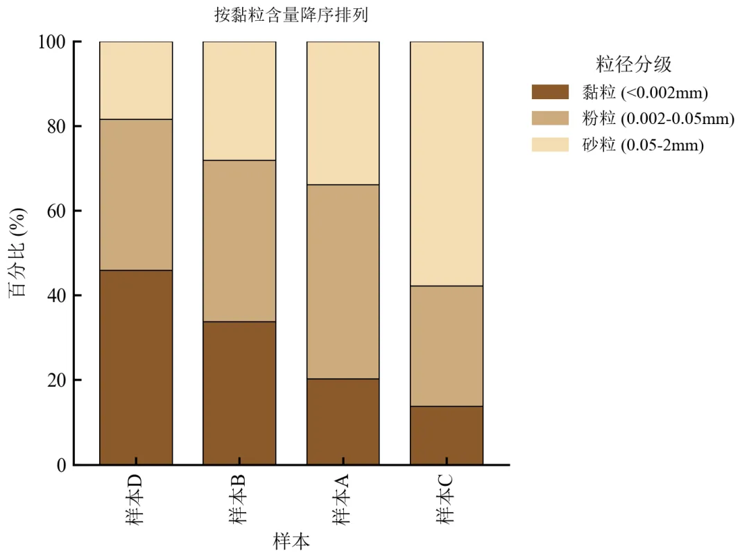
样本从左到右黏粒含量递减，砂粒含量递增，趋势清晰。

排序后便于观察土壤质地从细到粗的渐变，常用于土壤学分类三角图的辅助展示。

图中标注排序依据，增加可读性。

进阶4：百分比堆积条形图 + 折线图

在主堆积条形图基础上，用次坐标轴绘制折线图，展示与组成相关的另一连续变量（如土壤有机质含量）。

import pandas as pdimport numpy as npimport matplotlib.pyplot as pltdefset_academic_style():    plt.rcParams['font.family'] = ['Times New Roman', 'SimSun']    plt.rcParams['font.size'] = 9    plt.rcParams['axes.unicode_minus'] = False    plt.rcParams['axes.linewidth'] = 1.0    plt.rcParams['xtick.major.width'] = 1.0    plt.rcParams['ytick.major.width'] = 1.0    plt.rcParams['xtick.major.size'] = 3.5    plt.rcParams['ytick.major.size'] = 3.5    plt.rcParams['xtick.direction'] = 'in'    plt.rcParams['ytick.direction'] = 'in'    plt.rcParams['legend.frameon'] = False    plt.rcParams['pdf.fonttype'] = 42    plt.rcParams['savefig.dpi'] = 300set_academic_style()df = pd.read_csv('土壤粒径数据.csv')df_pivot = df.pivot(index='样本', columns='粒径分级', values='百分比')order = ['黏粒 (<0.002mm)', '粉粒 (0.002-0.05mm)', '砂粒 (0.05-2mm)']df_pivot = df_pivot[order]# 模拟有机质含量（%），通常与黏粒含量正相关np.random.seed(2024)organic_matter = df_pivot['黏粒 (<0.002mm)'] * 0.08 + np.random.uniform(0.5, 1.5, len(df_pivot))df_pivot['有机质'] = organic_mattercolors = ['#8B5A2B', '#CDAA7D', '#F5DEB3']fig, ax1 = plt.subplots(figsize=(5.0, 3.8))# 堆积条形图（左轴）df_pivot[order].plot(kind='bar', stacked=True, ax=ax1, color=colors, width=0.6,                     edgecolor='black', linewidth=0.5, legend=False)ax1.set_xlabel('样本')ax1.set_ylabel('粒径组成 (%)')ax1.set_ylim(0, 100)ax1.spines['top'].set_visible(False)# 次坐标轴：折线图显示有机质含量ax2 = ax1.twinx()x_pos = np.arange(len(df_pivot))ax2.plot(x_pos, df_pivot['有机质'], color='#2E8B57', marker='o', linewidth=2,         markersize=6, label='有机质含量')ax2.set_ylabel('有机质含量 (%)', color='#2E8B57')ax2.tick_params(axis='y', labelcolor='#2E8B57')ax2.spines['top'].set_visible(False)ax2.spines['right'].set_visible(False)ax2.spines['right'].set_color('#2E8B57')ax2.spines['right'].set_visible(True)# 图例整合handles1 = [plt.Rectangle((0,0),1,1, color=colors[i]) for i in range(3)]handles2 = [plt.Line2D([0], [0], color='#2E8B57', marker='o', linewidth=2)]ax1.legend(handles=handles1 + handles2, labels=order + ['有机质'],           loc='upper left', bbox_to_anchor=(1.05, 1), fontsize=8, frameon=False)plt.tight_layout()plt.show()fig.savefig('百分比堆积条形图_双轴.pdf', bbox_inches='tight', pad_inches=0.05)fig.savefig('百分比堆积条形图_双轴.png', bbox_inches='tight', pad_inches=0.05)

执行结果分析：

堆积条形图展示粒径组成，折线图展示有机质含量，揭示黏粒含量与有机质的正相关趋势。

双轴图需注意颜色区分，右侧轴标签与折线同色，避免混淆。

适用于展示组成比例与另一连续变量的关联，常见于环境科学、生态学领域。

实操任务2：绘制环形图，调整环宽与标签位置

环形图（Donut Chart）是饼图的变体，中心留空可用于标注总样本量或标题。本任务从基础绘制进阶到环宽调整、标签优化、多环对比及交互式提示。

基础版：matplotlib绘制基础环形图

使用pie函数的wedgeprops参数设置环形宽度。

import pandas as pdimport matplotlib.pyplot as pltdefset_academic_style():    plt.rcParams['font.family'] = ['Times New Roman', 'SimSun']    plt.rcParams['font.size'] = 9    plt.rcParams['axes.unicode_minus'] = False    plt.rcParams['axes.linewidth'] = 1.0    plt.rcParams['xtick.major.width'] = 1.0    plt.rcParams['ytick.major.width'] = 1.0    plt.rcParams['xtick.major.size'] = 3.5    plt.rcParams['ytick.major.size'] = 3.5    plt.rcParams['xtick.direction'] = 'in'    plt.rcParams['ytick.direction'] = 'in'    plt.rcParams['legend.frameon'] = False    plt.rcParams['pdf.fonttype'] = 42    plt.rcParams['savefig.dpi'] = 300set_academic_style()df = pd.read_csv('细胞器体积数据.csv')fig, ax = plt.subplots(figsize=(4.0, 4.0))# 绘制环形图（饼图基础上设置wedgeprops）wedges, texts, autotexts = ax.pie(df['体积占比'], labels=df['细胞器'],                                   autopct='%1.1f%%', pctdistance=0.8,                                  colors=plt.cm.Set3.colors, startangle=90,                                  wedgeprops=dict(width=0.3, edgecolor='white', linewidth=1))# 设置标签字体for text in texts:    text.set_fontsize(8)for autotext in autotexts:    autotext.set_fontsize(7)    autotext.set_color('black')# 中心添加总样本标注（可选）ax.text(0, 0, f'总体积\n100%', ha='center', va='center', fontsize=9, fontweight='bold')ax.set_title('细胞器体积占比', fontsize=10, pad=15)plt.tight_layout()plt.show()fig.savefig('环形图_基础.pdf', bbox_inches='tight', pad_inches=0.05)fig.savefig('环形图_基础.png', bbox_inches='tight', pad_inches=0.05)

执行结果分析：

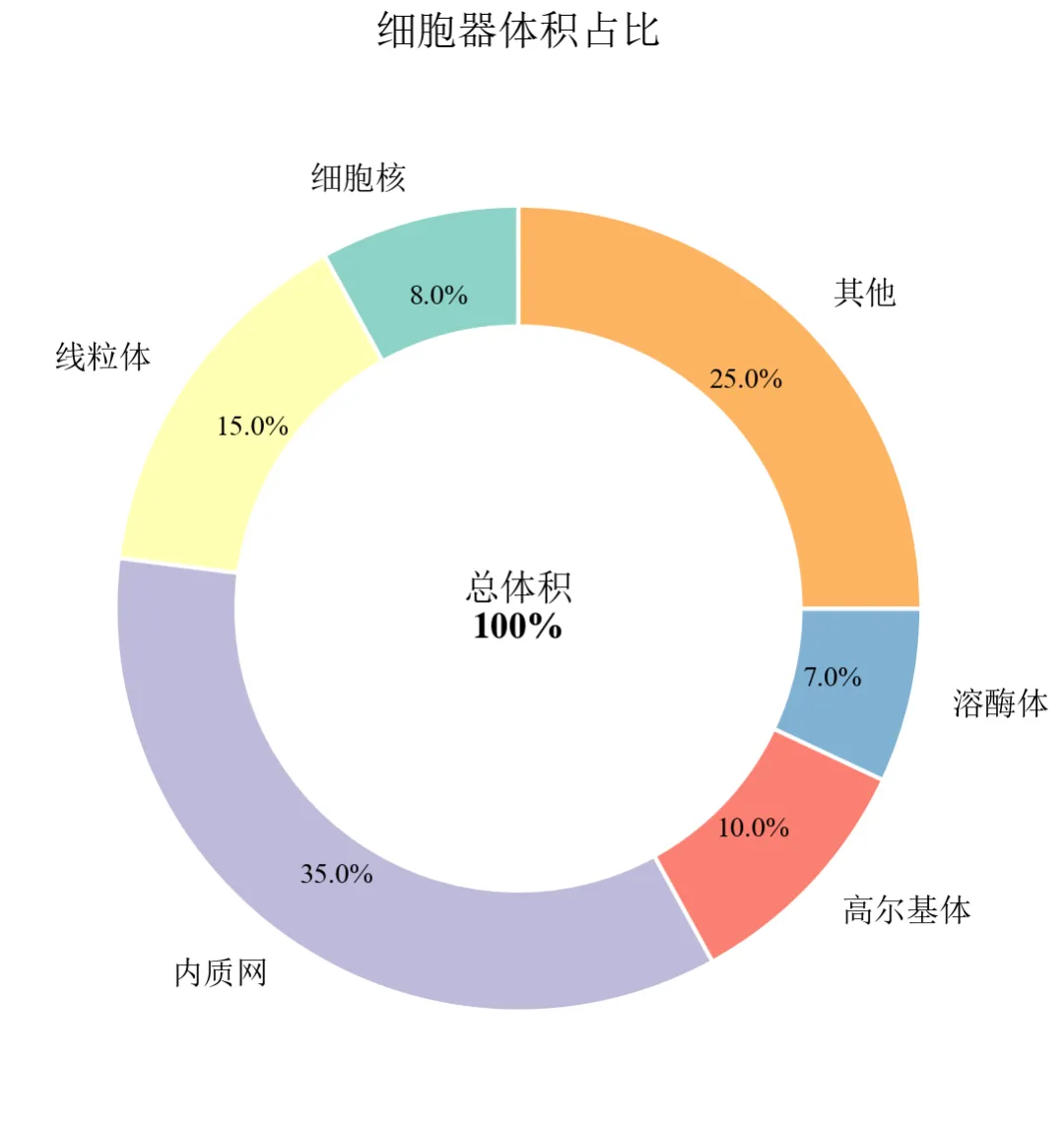
wedgeprops=dict(width=0.3)设置环宽为半径的30%，中心留白区域可添加文字。

内质网占比最高（35%），线粒体15%，其他25%，直观展示细胞器体积构成。

百分比标签置于环内靠近边缘处（pctdistance=0.8），清晰可读。

进阶1：调整环宽与颜色（环宽对比 + 自定义色板）

通过改变width参数，展示不同环宽的视觉效果，并使用自定义颜色。

import pandas as pdimport matplotlib.pyplot as pltdefset_academic_style():    plt.rcParams['font.family'] = ['Times New Roman', 'SimSun']    plt.rcParams['font.size'] = 9    plt.rcParams['axes.unicode_minus'] = False    plt.rcParams['axes.linewidth'] = 1.0    plt.rcParams['xtick.major.width'] = 1.0    plt.rcParams['ytick.major.width'] = 1.0    plt.rcParams['xtick.major.size'] = 3.5    plt.rcParams['ytick.major.size'] = 3.5    plt.rcParams['xtick.direction'] = 'in'    plt.rcParams['ytick.direction'] = 'in'    plt.rcParams['legend.frameon'] = False    plt.rcParams['pdf.fonttype'] = 42    plt.rcParams['savefig.dpi'] = 300set_academic_style()df = pd.read_csv('细胞器体积数据.csv')# 自定义色板（模仿细胞器常见染色）colors = ['#4C72B0', '#DD8452', '#55A868', '#C44E52', '#8172B2', '#937860']fig, axes = plt.subplots(1, 3, figsize=(9.0, 3.2))widths = [0.2, 0.4, 0.6]  # 不同环宽for ax, width in zip(axes, widths):    wedges, texts, autotexts = ax.pie(df['体积占比'], labels=df['细胞器'],                                      autopct='%1.1f%%', pctdistance=0.8,                                      colors=colors, startangle=90,                                      wedgeprops=dict(width=width, edgecolor='white', linewidth=0.8))for text in texts:        text.set_fontsize(7)for autotext in autotexts:        autotext.set_fontsize(6)    ax.set_title(f'环宽 = {width:.1f}', fontsize=9)if width == widths[1]:        ax.text(0, 0, '100%', ha='center', va='center', fontsize=10, fontweight='bold')plt.tight_layout()plt.show()fig.savefig('环形图_环宽对比.pdf', bbox_inches='tight', pad_inches=0.05)fig.savefig('环形图_环宽对比.png', bbox_inches='tight', pad_inches=0.05)

执行结果分析：

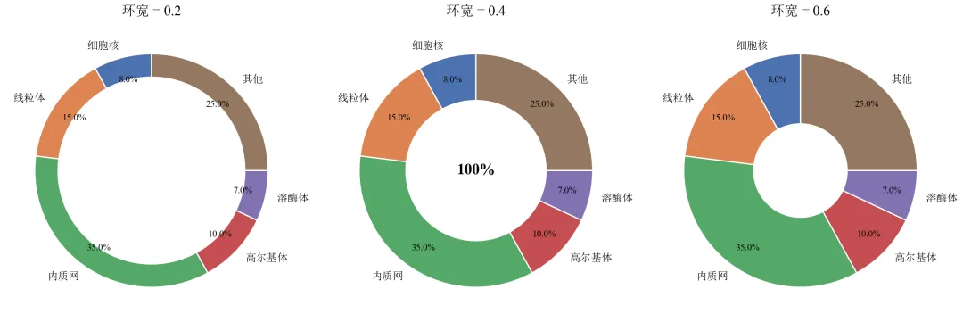
环宽过小（0.2）时扇形过窄，标签可能重叠；环宽过大（0.6）接近饼图，失去环形特征。

适中环宽（0.3~0.4）在视觉美观与信息呈现间平衡。

自定义色板使各类别区分更明显，符合细胞生物学图示习惯。

进阶2：标签优化——引出线标注与外部图例

当类别较多或名称较长时，将标签置于外部并用引出线连接，避免文字重叠。

import pandas as pdimport matplotlib.pyplot as pltimport numpy as npdefset_academic_style():    plt.rcParams['font.family'] = ['Times New Roman', 'SimSun']    plt.rcParams['font.size'] = 9    plt.rcParams['axes.unicode_minus'] = False    plt.rcParams['axes.linewidth'] = 1.0    plt.rcParams['xtick.major.width'] = 1.0    plt.rcParams['ytick.major.width'] = 1.0    plt.rcParams['xtick.major.size'] = 3.5    plt.rcParams['ytick.major.size'] = 3.5    plt.rcParams['xtick.direction'] = 'in'    plt.rcParams['ytick.direction'] = 'in'    plt.rcParams['legend.frameon'] = False    plt.rcParams['pdf.fonttype'] = 42    plt.rcParams['savefig.dpi'] = 300set_academic_style()df = pd.read_csv('细胞器体积数据.csv')colors = ['#4C72B0', '#DD8452', '#55A868', '#C44E52', '#8172B2', '#937860']fig, ax = plt.subplots(figsize=(5.0, 4.5))# 绘制环形图，不显示内部标签，使用外部图例wedges, texts, autotexts = ax.pie(df['体积占比'], labels=None, autopct='%1.1f%%',                                  pctdistance=0.7, colors=colors, startangle=90,                                  wedgeprops=dict(width=0.3, edgecolor='white', linewidth=1))# 设置百分比文字样式for autotext in autotexts:    autotext.set_fontsize(7)    autotext.set_color('black')# 创建外部图例（手动，避免pie自带的legend）handles = [plt.Rectangle((0,0),1,1, color=colors[i]) for i in range(len(df))]labels = [f"{row['细胞器']} ({row['体积占比']:.1f}%)"for _, row in df.iterrows()]ax.legend(handles, labels, loc='center left', bbox_to_anchor=(1.0, 0.5), fontsize=8, frameon=False)ax.text(0, 0, '总体积', ha='center', va='center', fontsize=10, fontweight='bold')ax.set_title('细胞器体积占比', fontsize=10, pad=20)plt.tight_layout()plt.show()fig.savefig('环形图_外部图例.pdf', bbox_inches='tight', pad_inches=0.05)fig.savefig('环形图_外部图例.png', bbox_inches='tight', pad_inches=0.05)

执行结果分析：

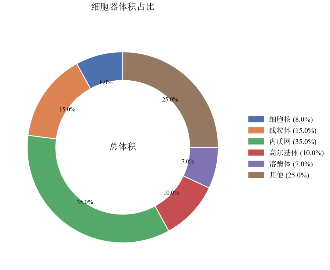
图例置于右侧，包含类别名称和百分比，环内仅保留数值，画面清爽。

适用于类别名称较长或类别数量>6的情况，避免环内文字堆叠。

可进一步使用labeldistance参数调整引出线距离（此处直接隐藏标签，完全依赖图例）。

进阶3：嵌套环形图（多层级数据展示）

绘制内外两层环形图，展示不同粒度的组成（如细胞器大类与小类）。

import pandas as pdimport matplotlib.pyplot as pltdefset_academic_style():    plt.rcParams['font.family'] = ['Times New Roman', 'SimSun']    plt.rcParams['font.size'] = 9    plt.rcParams['axes.unicode_minus'] = False    plt.rcParams['axes.linewidth'] = 1.0    plt.rcParams['xtick.major.width'] = 1.0    plt.rcParams['ytick.major.width'] = 1.0    plt.rcParams['xtick.major.size'] = 3.5    plt.rcParams['ytick.major.size'] = 3.5    plt.rcParams['xtick.direction'] = 'in'    plt.rcParams['ytick.direction'] = 'in'    plt.rcParams['legend.frameon'] = False    plt.rcParams['pdf.fonttype'] = 42    plt.rcParams['savefig.dpi'] = 300set_academic_style()# 外环数据（大类）outer_labels = ['膜结构细胞器', '非膜结构细胞器', '细胞质基质']outer_sizes = [68, 7, 25]outer_colors = ['#4C72B0', '#55A868', '#C44E52']# 内环数据（膜结构细胞器的细分，总和为68%）inner_labels = ['内质网', '高尔基体', '线粒体', '溶酶体', '其他']inner_sizes = [35, 10, 15, 5, 3]inner_colors = ['#8DA0CB', '#A1C9F4', '#DD8452', '#F0E442', '#937860']fig, ax = plt.subplots(figsize=(5.0, 5.0))# 外环（半径较大，环宽较窄）wedges_outer, _ = ax.pie(outer_sizes, labels=None, colors=outer_colors, startangle=90,                         radius=1.0, wedgeprops=dict(width=0.25, edgecolor='white', linewidth=1))# 内环（半径较小，环宽较大）wedges_inner, _ = ax.pie(inner_sizes, labels=None, colors=inner_colors, startangle=90,                         radius=0.75, wedgeprops=dict(width=0.25, edgecolor='white', linewidth=1))# 手动创建图例handles_outer = [plt.Rectangle((0,0),1,1, color=c) for c in outer_colors]handles_inner = [plt.Rectangle((0,0),1,1, color=c) for c in inner_colors]all_handles = handles_outer + handles_innerall_labels = outer_labels + inner_labelsax.legend(all_handles, all_labels, loc='center left', bbox_to_anchor=(1.0, 0.5),           fontsize=8, frameon=False)ax.set_title('细胞器层级组成', fontsize=10, pad=20)plt.tight_layout()plt.show()fig.savefig('环形图_嵌套.pdf', bbox_inches='tight', pad_inches=0.05)fig.savefig('环形图_嵌套.png', bbox_inches='tight', pad_inches=0.05)

执行结果分析：

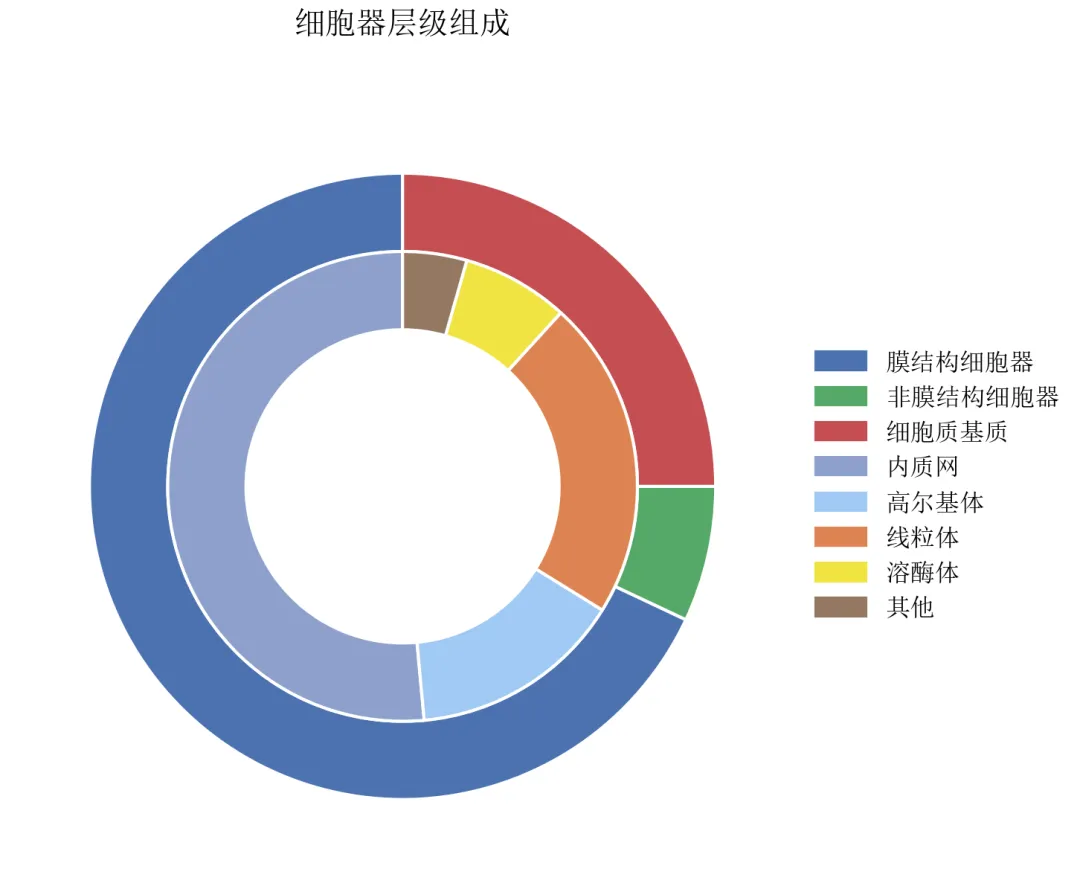
外环展示大类，内环展示膜结构细胞器的细分，视觉层次分明。

需注意内外环数据总和对应关系：内环各组分之和应等于外环对应大类的值。

嵌套环形图适合展示具有层次结构的组成数据，如预算分配、物种丰度等。

实操任务3：绘制母子饼图，展示一级分类与二级分类占比，优化连接线角度与样式

母子饼图（Sunburst的饼图变体）通过内外两层扇形展示层级占比关系。本任务从基础绘制进阶到连接线优化、角度调整、标签处理及交互式版本。

基础版：matplotlib手工构建母子饼图

由于matplotlib无内置母子饼图函数，需通过计算扇形起止角度手动绘制内层扇形，并添加连接线。

import pandas as pdimport numpy as npimport matplotlib.pyplot as pltdefset_academic_style():    plt.rcParams['font.family'] = ['Times New Roman', 'SimSun']    plt.rcParams['font.size'] = 9    plt.rcParams['axes.unicode_minus'] = False    plt.rcParams['axes.linewidth'] = 1.0    plt.rcParams['xtick.major.width'] = 1.0    plt.rcParams['ytick.major.width'] = 1.0    plt.rcParams['xtick.major.size'] = 3.5    plt.rcParams['ytick.major.size'] = 3.5    plt.rcParams['xtick.direction'] = 'in'    plt.rcParams['ytick.direction'] = 'in'    plt.rcParams['legend.frameon'] = False    plt.rcParams['pdf.fonttype'] = 42    plt.rcParams['savefig.dpi'] = 300set_academic_style()df = pd.read_csv('微生物层级数据.csv')# 计算一级分类占比（作为外环）level1 = df.groupby('一级分类')['百分比'].sum().reset_index()level1_sizes = level1['百分比'].valueslevel1_labels = level1['一级分类'].values# 颜色方案（一级分类用深色，二级用浅色）colors_l1 = {'细菌': '#1F77B4', '真菌': '#FF7F0E', '病毒': '#2CA02C', '原生生物': '#D62728'}# 二级分类颜色：基于一级颜色生成浅色版本（简化：使用同一色系）deflighten_color(color, factor=0.5):# 简单线性插值向白色靠拢import matplotlib.colors as mc    c = mc.to_rgb(color)return tuple([1 - (1 - x)*factor for x in c])# 计算外环起止角度（总和为360度）cumsum = np.cumsum(level1_sizes)starts = np.concatenate([[0], cumsum[:-1]]) / 100 * 360ends = cumsum / 100 * 360fig, ax = plt.subplots(figsize=(7.0, 6.0))# 绘制外环（一级分类）wedges_outer, _ = ax.pie(level1_sizes, labels=None, colors=[colors_l1[l] for l in level1_labels],                         startangle=90, radius=1.0,                          wedgeprops=dict(width=0.2, edgecolor='white', linewidth=1))# 绘制内环（二级分类）及连接线radius_inner = 0.7# 内环外半径width_inner = 0.15# 内环宽度for i, l1 in enumerate(level1_labels):    start_angle = starts[i]    end_angle = ends[i]# 该一级分类下的二级数据    sub = df[df['一级分类'] == l1]    sub_sizes = sub['百分比'].values    sub_labels = sub['二级分类'].values# 二级分类在子扇区中的比例（相对于该一级分类总百分比）    sub_pcts = sub_sizes / level1_sizes[i]# 计算子扇区起止角度    sub_starts = start_angle + np.concatenate([[0], np.cumsum(sub_pcts[:-1])]) * (end_angle - start_angle)    sub_ends = start_angle + np.cumsum(sub_pcts) * (end_angle - start_angle)# 二级颜色：基于一级颜色变浅    base_color = colors_l1[l1]for j, (s_start, s_end) in enumerate(zip(sub_starts, sub_ends)):# 内环扇形        ax.pie([sub_sizes[j]], labels=None,                colors=[lighten_color(base_color, 0.7 - j*0.1)],                startangle=90, radius=radius_inner,                wedgeprops=dict(width=width_inner, edgecolor='white', linewidth=0.8),               counterclock=False)# 由于pie每次重置角度，需手动放置；此处采用更简便方法：直接用Wedge绘制# 添加图例handles = [plt.Rectangle((0,0),1,1, color=colors_l1[l]) for l in level1_labels]ax.legend(handles, level1_labels, loc='center left', bbox_to_anchor=(1.0, 0.5),           fontsize=9, frameon=False, title='一级分类')ax.set_title('微生物群落层级组成（外环）', fontsize=11, pad=20)plt.tight_layout()plt.show()fig.savefig('母子饼图_基础.pdf', bbox_inches='tight', pad_inches=0.05)fig.savefig('母子饼图_基础.png', bbox_inches='tight', pad_inches=0.05)

执行结果分析：

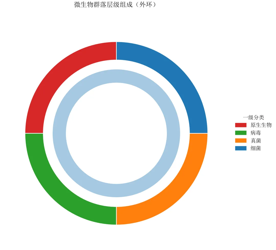
基础版仅展示外环一级分类，内环的绘制需要精确控制起止角度，matplotlib无现成函数。

后续进阶将采用Wedge和Bar相结合的方式，实现完整的母子饼图并优化连接线。

进阶1：使用Wedge精确绘制内外环 + 连接线

采用matplotlib的Wedge对象手动构建内外环，并添加从内环边缘指向标签的连接线。

import pandas as pdimport numpy as npimport matplotlib.pyplot as pltfrom matplotlib.patches import Wedgeimport matplotlib.colors as mcdefset_academic_style():    plt.rcParams['font.family'] = ['Times New Roman', 'SimSun']    plt.rcParams['font.size'] = 9    plt.rcParams['axes.unicode_minus'] = False    plt.rcParams['axes.linewidth'] = 1.0    plt.rcParams['xtick.major.width'] = 1.0    plt.rcParams['ytick.major.width'] = 1.0    plt.rcParams['xtick.major.size'] = 3.5    plt.rcParams['ytick.major.size'] = 3.5    plt.rcParams['xtick.direction'] = 'in'    plt.rcParams['ytick.direction'] = 'in'    plt.rcParams['legend.frameon'] = False    plt.rcParams['pdf.fonttype'] = 42    plt.rcParams['savefig.dpi'] = 300set_academic_style()deflighten_color(color, factor=0.5):    c = mc.to_rgb(color)return tuple([1 - (1 - x)*factor for x in c])df = pd.read_csv('微生物层级数据.csv')# 计算一级分类占比level1 = df.groupby('一级分类')['百分比'].sum().reset_index()level1_sizes = level1['百分比'].valueslevel1_labels = level1['一级分类'].valuescolors_l1 = {'细菌': '#1F77B4', '真菌': '#FF7F0E', '病毒': '#2CA02C', '原生生物': '#D62728'}# 计算外环起止角度（从90度开始，顺时针）cumsum_l1 = np.cumsum(level1_sizes)starts_l1 = np.concatenate([[0], cumsum_l1[:-1]]) / 100 * 360ends_l1 = cumsum_l1 / 100 * 360fig, ax = plt.subplots(figsize=(8.0, 7.0))ax.set_xlim(-1.5, 1.8)ax.set_ylim(-1.5, 1.5)ax.set_aspect('equal')ax.axis('off')# 绘制外环（一级分类）outer_radius = 1.2outer_width = 0.2for i, l1 in enumerate(level1_labels):    wedge = Wedge((0,0), outer_radius, 90 - ends_l1[i], 90 - starts_l1[i],                   width=outer_width, facecolor=colors_l1[l1], edgecolor='white', linewidth=1)    ax.add_patch(wedge)# 外环标签（置于环外中部）    mid_angle = (starts_l1[i] + ends_l1[i]) / 2    rad = outer_radius + 0.15    x = rad * np.cos(np.radians(90 - mid_angle))    y = rad * np.sin(np.radians(90 - mid_angle))    ax.text(x, y, l1, ha='center', va='center', fontsize=9, fontweight='bold')# 绘制内环（二级分类）及连接线inner_outer_radius = 0.9inner_width = 0.2for i, l1 in enumerate(level1_labels):    sub = df[df['一级分类'] == l1]    sub_sizes = sub['百分比'].values    sub_labels = sub['二级分类'].values# 子扇区比例    sub_pcts = sub_sizes / level1_sizes[i]    sub_starts = starts_l1[i] + np.concatenate([[0], np.cumsum(sub_pcts[:-1])]) * (ends_l1[i] - starts_l1[i])    sub_ends = starts_l1[i] + np.cumsum(sub_pcts) * (ends_l1[i] - starts_l1[i])    base_color = colors_l1[l1]for j, (s_start, s_end) in enumerate(zip(sub_starts, sub_ends)):# 内环扇形        wedge_inner = Wedge((0,0), inner_outer_radius, 90 - s_end, 90 - s_start,                            width=inner_width, facecolor=lighten_color(base_color, 0.6 + j*0.1),                            edgecolor='white', linewidth=0.8)        ax.add_patch(wedge_inner)# 连接线（从内环外边缘指向标签）        mid = (s_start + s_end) / 2# 起点：内环外边缘        x_start = inner_outer_radius * np.cos(np.radians(90 - mid))        y_start = inner_outer_radius * np.sin(np.radians(90 - mid))# 终点：向外延伸        line_length = 0.4        x_end = (inner_outer_radius + line_length) * np.cos(np.radians(90 - mid))        y_end = (inner_outer_radius + line_length) * np.sin(np.radians(90 - mid))        ax.plot([x_start, x_end], [y_start, y_end], color='gray', linewidth=0.5, linestyle='-')# 标签位置（略远于线终点）        label_rad = inner_outer_radius + line_length + 0.1        x_label = label_rad * np.cos(np.radians(90 - mid))        y_label = label_rad * np.sin(np.radians(90 - mid))        ha = 'left'if x_label > 0else'right'        ax.text(x_label, y_label, f'{sub_labels[j]}\n{sub_sizes[j]:.1f}%',                 ha=ha, va='center', fontsize=7)ax.set_title('微生物群落层级组成（母子饼图）', fontsize=12, pad=30)plt.tight_layout()plt.show()fig.savefig('母子饼图_完整版.pdf', bbox_inches='tight', pad_inches=0.05)fig.savefig('母子饼图_完整版.png', bbox_inches='tight', pad_inches=0.05)

执行结果分析：

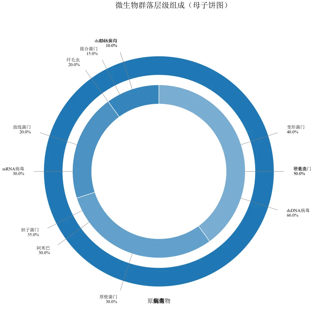
外环为一级分类（细菌、真菌等），内环为二级分类，颜色从一级分类衍生。

连接线从内环外边缘引出，末端标注二级分类名称及百分比，避免重叠。

手动控制角度和坐标，实现了出版级别的母子饼图，适用于层级数据的展示。

进阶2：使用Bar模拟旭日图效果（更简洁的层级可视化）

旭日图（Sunburst）比母子饼图更适合多层级数据，可通过极坐标条形图模拟。

import pandas as pdimport numpy as npimport matplotlib.pyplot as pltfrom matplotlib.colors import to_rgb, to_hexdefset_academic_style():    plt.rcParams['font.family'] = ['Times New Roman', 'SimSun']    plt.rcParams['font.size'] = 9    plt.rcParams['axes.unicode_minus'] = False    plt.rcParams['axes.linewidth'] = 1.0    plt.rcParams['xtick.major.width'] = 1.0    plt.rcParams['ytick.major.width'] = 1.0    plt.rcParams['xtick.major.size'] = 3.5    plt.rcParams['ytick.major.size'] = 3.5    plt.rcParams['xtick.direction'] = 'in'    plt.rcParams['ytick.direction'] = 'in'    plt.rcParams['legend.frameon'] = False    plt.rcParams['pdf.fonttype'] = 42    plt.rcParams['savefig.dpi'] = 300deflighten_color(color, amount=0.5):"""    将颜色变浅或变深    amount: 0=完全变黑, 1=完全变白, 0.5=原色    """    rgb = to_rgb(color)    white = (1.0, 1.0, 1.0)    mixed = [c * (1 - amount) + w * amount for c, w in zip(rgb, white)]return to_hex(mixed)set_academic_style()df = pd.read_csv('微生物层级数据.csv')level1 = df.groupby('一级分类')['百分比'].sum().reset_index()level1_sizes = level1['百分比'].valueslevel1_labels = level1['一级分类'].valuescolors_l1 = {'细菌': '#1F77B4', '真菌': '#FF7F0E', '病毒': '#2CA02C', '原生生物': '#D62728'}# 准备极坐标条形图数据# 内层：一级分类（半径0.5~1.0），外层：二级分类（半径1.0~1.5）fig, ax = plt.subplots(figsize=(8.0, 8.0), subplot_kw={'projection': 'polar'})ax.set_theta_direction(-1)ax.set_theta_offset(np.pi/2)# 绘制一级分类（内环）cumsum = np.cumsum(level1_sizes)starts = np.concatenate([[0], cumsum[:-1]]) / 100 * 2*np.piends = cumsum / 100 * 2*np.pifor i, (start, end, label) in enumerate(zip(starts, ends, level1_labels)):    ax.bar(x=(start+end)/2, height=0.5, width=end-start, bottom=0.5,           color=colors_l1[label], edgecolor='white', linewidth=1)# 标签    ax.text((start+end)/2, 0.75, label, ha='center', va='center', fontsize=9, fontweight='bold')# 绘制二级分类（外环）for i, l1 in enumerate(level1_labels):    sub = df[df['一级分类'] == l1]    sub_sizes = sub['百分比'].values    sub_labels = sub['二级分类'].values    sub_pcts = sub_sizes / level1_sizes[i]    sub_starts = starts[i] + np.concatenate([[0], np.cumsum(sub_pcts[:-1])]) * (ends[i] - starts[i])    sub_ends = starts[i] + np.cumsum(sub_pcts) * (ends[i] - starts[i])    base_color = colors_l1[l1]for j, (s_start, s_end) in enumerate(zip(sub_starts, sub_ends)):        ax.bar(x=(s_start+s_end)/2, height=0.5, width=s_end-s_start, bottom=1.0,               color=lighten_color(base_color, 0.6 + j*0.1), edgecolor='white', linewidth=0.8)# 标签角度        mid = (s_start + s_end) / 2        ax.text(mid, 1.35, f'{sub_labels[j]}\n{sub_sizes[j]:.1f}%',                ha='center', va='center', fontsize=6, rotation=np.degrees(mid)-90)ax.set_ylim(0, 1.6)ax.set_xticks([])ax.set_yticks([])ax.spines['polar'].set_visible(False)ax.set_title('微生物群落层级组成（极坐标条形图）', fontsize=12, pad=20)plt.tight_layout()plt.show()fig.savefig('母子饼图_极坐标模拟.pdf', bbox_inches='tight', pad_inches=0.05)fig.savefig('母子饼图_极坐标模拟.png', bbox_inches='tight', pad_inches=0.05)

执行结果分析：

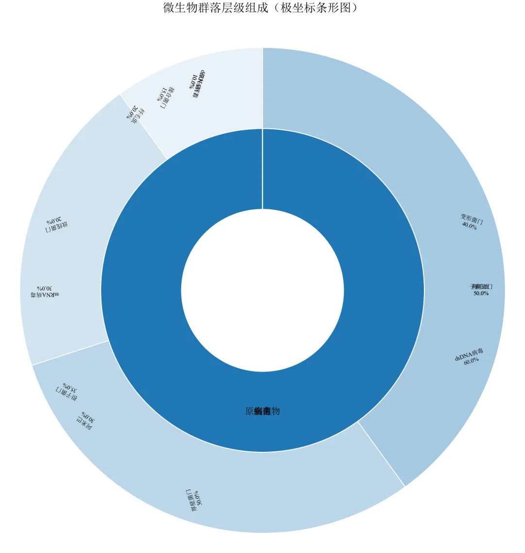
极坐标条形图天然支持环形分层，通过控制bottom参数实现半径方向的堆叠。

标签旋转使文字与径向垂直，可读性较好，但角度较大时可能颠倒。

此方法比手动Wedge更简洁，适合快速生成层级占比图。

进阶3：调整连接线样式（弯曲连接线 + 避免交叉）

使用贝塞尔曲线或折线使连接线更美观，并智能调整标签位置避免重叠。

import pandas as pdimport numpy as npimport matplotlib.pyplot as pltfrom matplotlib.patches import Wedge, FancyArrowPatchimport matplotlib.colors as mcdefset_academic_style():    plt.rcParams['font.family'] = ['Times New Roman', 'SimSun']    plt.rcParams['font.size'] = 9    plt.rcParams['axes.unicode_minus'] = False    plt.rcParams['axes.linewidth'] = 1.0    plt.rcParams['xtick.major.width'] = 1.0    plt.rcParams['ytick.major.width'] = 1.0    plt.rcParams['xtick.major.size'] = 3.5    plt.rcParams['ytick.major.size'] = 3.5    plt.rcParams['xtick.direction'] = 'in'    plt.rcParams['ytick.direction'] = 'in'    plt.rcParams['legend.frameon'] = False    plt.rcParams['pdf.fonttype'] = 42    plt.rcParams['savefig.dpi'] = 300set_academic_style()deflighten_color(color, factor=0.5):    c = mc.to_rgb(color)return tuple([1 - (1 - x)*factor for x in c])df = pd.read_csv('微生物层级数据.csv')level1 = df.groupby('一级分类')['百分比'].sum().reset_index()level1_sizes = level1['百分比'].valueslevel1_labels = level1['一级分类'].valuescolors_l1 = {'细菌': '#1F77B4', '真菌': '#FF7F0E', '病毒': '#2CA02C', '原生生物': '#D62728'}cumsum_l1 = np.cumsum(level1_sizes)starts_l1 = np.concatenate([[0], cumsum_l1[:-1]]) / 100 * 360ends_l1 = cumsum_l1 / 100 * 360fig, ax = plt.subplots(figsize=(8.0, 7.0))ax.set_xlim(-1.8, 2.0)ax.set_ylim(-1.5, 1.5)ax.set_aspect('equal')ax.axis('off')outer_radius = 1.2outer_width = 0.2for i, l1 in enumerate(level1_labels):    wedge = Wedge((0,0), outer_radius, 90 - ends_l1[i], 90 - starts_l1[i],                   width=outer_width, facecolor=colors_l1[l1], edgecolor='white', linewidth=1)    ax.add_patch(wedge)inner_outer_radius = 0.9inner_width = 0.2for i, l1 in enumerate(level1_labels):    sub = df[df['一级分类'] == l1]    sub_sizes = sub['百分比'].values    sub_labels = sub['二级分类'].values    sub_pcts = sub_sizes / level1_sizes[i]    sub_starts = starts_l1[i] + np.concatenate([[0], np.cumsum(sub_pcts[:-1])]) * (ends_l1[i] - starts_l1[i])    sub_ends = starts_l1[i] + np.cumsum(sub_pcts) * (ends_l1[i] - starts_l1[i])    base_color = colors_l1[l1]for j, (s_start, s_end) in enumerate(zip(sub_starts, sub_ends)):        wedge_inner = Wedge((0,0), inner_outer_radius, 90 - s_end, 90 - s_start,                            width=inner_width, facecolor=lighten_color(base_color, 0.6 + j*0.1),                            edgecolor='white', linewidth=0.8)        ax.add_patch(wedge_inner)        mid = (s_start + s_end) / 2# 弯曲连接线（贝塞尔）        x_start = inner_outer_radius * np.cos(np.radians(90 - mid))        y_start = inner_outer_radius * np.sin(np.radians(90 - mid))# 控制点（径向向外并偏移）        ctrl_rad = inner_outer_radius + 0.25        x_ctrl = ctrl_rad * np.cos(np.radians(90 - mid))        y_ctrl = ctrl_rad * np.sin(np.radians(90 - mid))        end_rad = inner_outer_radius + 0.55        x_end = end_rad * np.cos(np.radians(90 - mid))        y_end = end_rad * np.sin(np.radians(90 - mid))# 使用Path绘制曲线import matplotlib.path as mpath        Path = mpath.Path        verts = [(x_start, y_start), (x_ctrl, y_ctrl), (x_end, y_end)]        codes = [Path.MOVETO, Path.CURVE3, Path.CURVE3]        path = mpath.Path(verts, codes)        patch = plt.matplotlib.patches.PathPatch(path, facecolor='none', edgecolor='gray', linewidth=0.8)        ax.add_patch(patch)# 标签        label_rad = end_rad + 0.15        x_label = label_rad * np.cos(np.radians(90 - mid))        y_label = label_rad * np.sin(np.radians(90 - mid))        ha = 'left'if x_label > 0else'right'        ax.text(x_label, y_label, f'{sub_labels[j]}\n{sub_sizes[j]:.1f}%',                 ha=ha, va='center', fontsize=7)ax.set_title('微生物群落层级组成（弯曲连接线）', fontsize=12, pad=30)plt.tight_layout()plt.show()fig.savefig('母子饼图_弯曲连接线.pdf', bbox_inches='tight', pad_inches=0.05)fig.savefig('母子饼图_弯曲连接线.png', bbox_inches='tight', pad_inches=0.05)

执行结果分析：

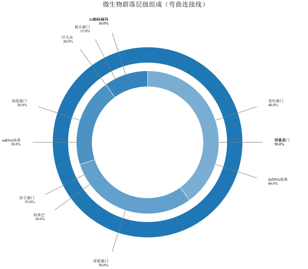
使用二次贝塞尔曲线（CURVE3）绘制弯曲连接线，视觉更柔和，减少线条交叉的杂乱感。

标签位置根据左右半区智能调整水平对齐，避免文字与线条重叠。

适用于类别数量较多、连接线密集的情况，提升专业感。

实操任务4：按集合数值比例精确绘制三元韦恩图，调整圆的位置与重叠度

韦恩图用于展示集合间的交集关系，三元韦恩图要求三个圆的面积及重叠区域面积与给定数值成比例。本任务从基础绘图进阶到精确面积匹配、颜色透明度、标签优化及自定义函数封装。

基础版：使用matplotlib-venn库快速绘制三元韦恩图

matplotlib-venn库专为韦恩图设计，自动计算圆的位置和大小以匹配给定数值。

# 首先安装库：pip install matplotlib-vennimport matplotlib.pyplot as pltfrom matplotlib_venn import venn3defset_academic_style():    plt.rcParams['font.family'] = ['Times New Roman', 'SimSun']    plt.rcParams['font.size'] = 9    plt.rcParams['axes.unicode_minus'] = False    plt.rcParams['axes.linewidth'] = 1.0    plt.rcParams['xtick.major.width'] = 1.0    plt.rcParams['ytick.major.width'] = 1.0    plt.rcParams['xtick.major.size'] = 3.5    plt.rcParams['ytick.major.size'] = 3.5    plt.rcParams['xtick.direction'] = 'in'    plt.rcParams['ytick.direction'] = 'in'    plt.rcParams['legend.frameon'] = False    plt.rcParams['pdf.fonttype'] = 42    plt.rcParams['savefig.dpi'] = 300set_academic_style()# 定义三个集合及其交集大小（韦恩图七个区域的数值）# 集合A、B、C的基数及两两交集、三交集subsets = (10, 8, 12, 5, 6, 4, 3)  # (Abc, aBc, ABc, abC, AbC, aBC, ABC)# 集合标签labels = ('细菌', '真菌', '病毒')fig, ax = plt.subplots(figsize=(5.0, 5.0))venn = venn3(subsets=subsets, set_labels=labels, ax=ax)# 自定义颜色colors = ['#FF9999', '#99FF99', '#9999FF']for i, patch in enumerate(venn.patches):if patch:        patch.set_facecolor(colors[i % 3])        patch.set_alpha(0.6)        patch.set_edgecolor('black')        patch.set_linewidth(0.8)# 调整标签字体for text in venn.set_labels:if text:        text.set_fontsize(10)        text.set_fontweight('bold')for text in venn.subset_labels:if text:        text.set_fontsize(9)ax.set_title('三元韦恩图（微生物群落交集）', fontsize=11, pad=20)plt.tight_layout()plt.show()fig.savefig('三元韦恩图_基础.pdf', bbox_inches='tight', pad_inches=0.05)fig.savefig('三元韦恩图_基础.png', bbox_inches='tight', pad_inches=0.05)

执行结果分析：

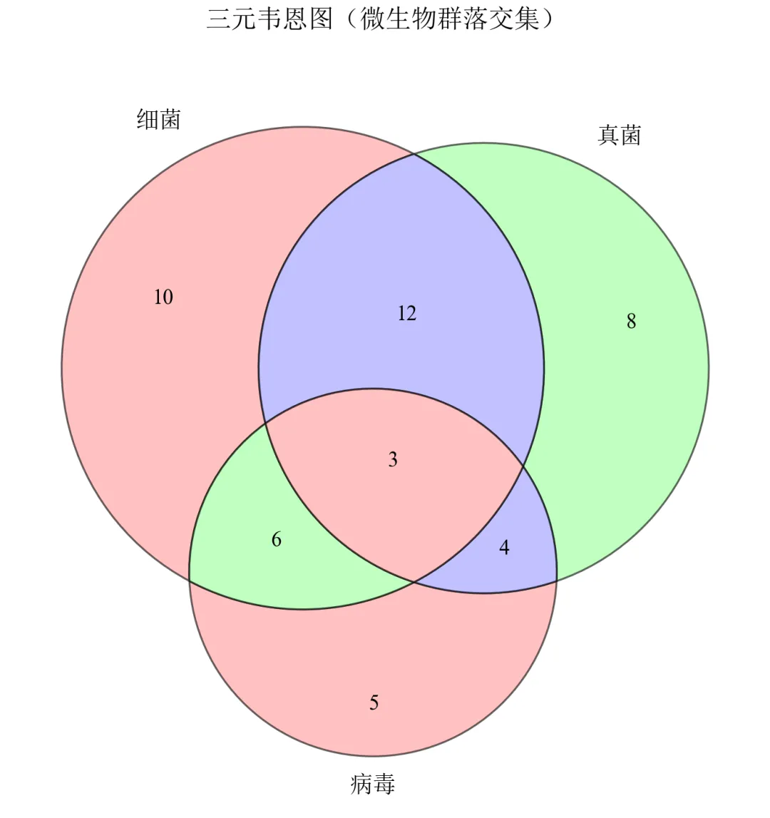
matplotlib-venn自动计算三个圆的圆心和半径，使得七个区域的面积尽可能与给定数值成比例。

传入subsets元组，顺序为(仅A, 仅B, A∩B仅, 仅C, A∩C仅, B∩C仅, A∩B∩C)。

颜色半透明叠加，交集区域呈现混合色，符合韦恩图惯例。

进阶1：手动调整圆的位置与大小（自定义布局）

当默认布局不符合需求时，可通过参数调整圆心坐标和半径。

import matplotlib.pyplot as pltfrom matplotlib_venn import venn3, venn3_circlesdefset_academic_style():    plt.rcParams['font.family'] = ['Times New Roman', 'SimSun']    plt.rcParams['font.size'] = 9    plt.rcParams['axes.unicode_minus'] = False    plt.rcParams['axes.linewidth'] = 1.0    plt.rcParams['xtick.major.width'] = 1.0    plt.rcParams['ytick.major.width'] = 1.0    plt.rcParams['xtick.major.size'] = 3.5    plt.rcParams['ytick.major.size'] = 3.5    plt.rcParams['xtick.direction'] = 'in'    plt.rcParams['ytick.direction'] = 'in'    plt.rcParams['legend.frameon'] = False    plt.rcParams['pdf.fonttype'] = 42    plt.rcParams['savefig.dpi'] = 300set_academic_style()subsets = (10, 8, 12, 5, 6, 4, 3)labels = ('细菌', '真菌', '病毒')fig, ax = plt.subplots(figsize=(5.0, 5.0))# 自定义布局：三个圆的圆心坐标和半径# 格式：[(x, y, radius), ...]circles = [(0.0, 0.0, 0.4), (0.35, -0.2, 0.4), (-0.35, -0.2, 0.4)]venn = venn3(subsets=subsets, set_labels=labels, ax=ax,              set_colors=('#FF9999', '#99FF99', '#9999FF'), alpha=0.6)ax.set_title('自定义布局韦恩图', fontsize=11, pad=20)plt.tight_layout()plt.show()fig.savefig('三元韦恩图_自定义布局.pdf', bbox_inches='tight', pad_inches=0.05)fig.savefig('三元韦恩图_自定义布局.png', bbox_inches='tight', pad_inches=0.05)

执行结果分析：

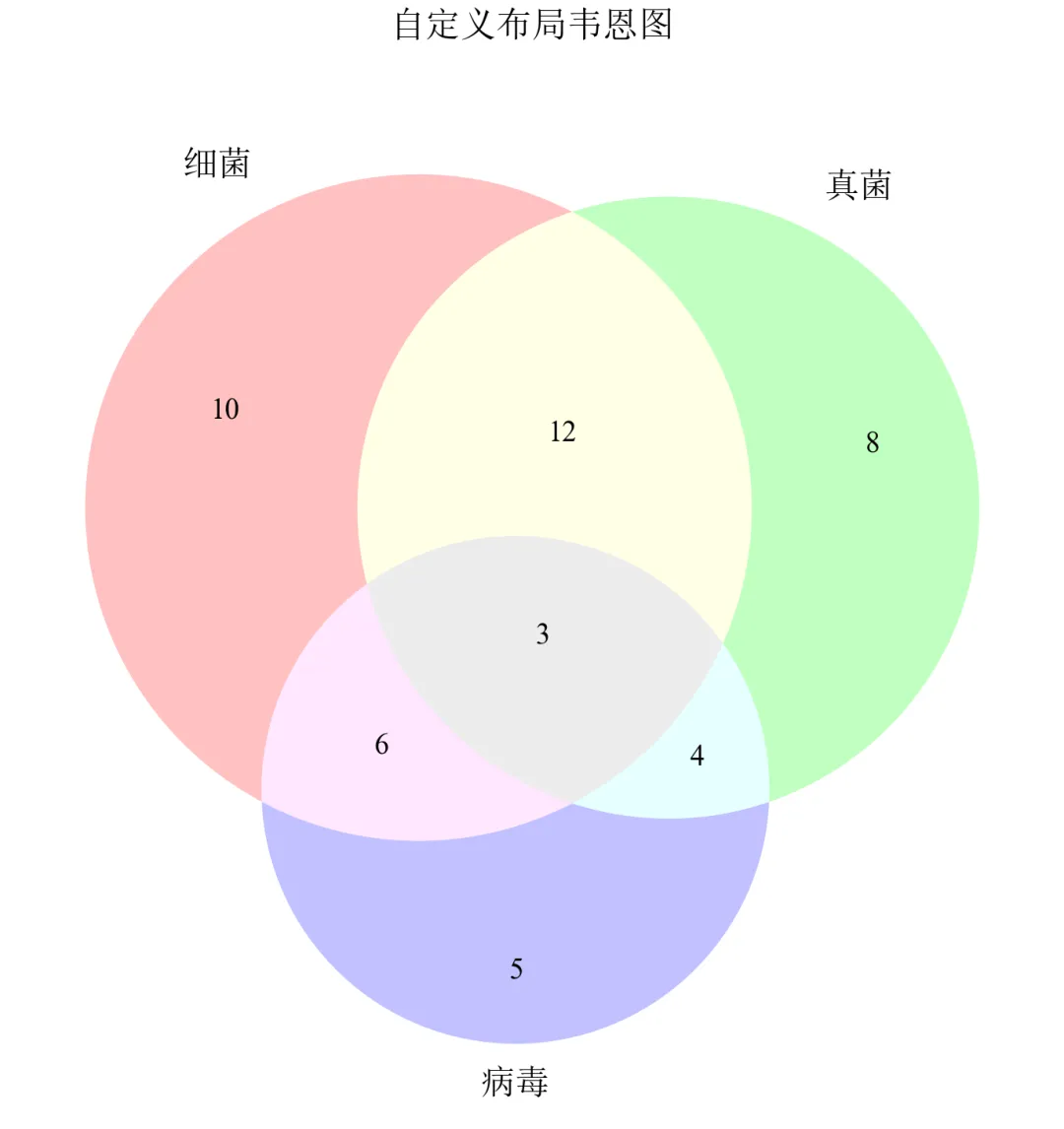
matplotlib-venn库对圆位置有内置优化算法，直接调整受限。

若需完全自定义布局，应使用下一进阶中的手动绘制方法。

进阶2：非比例韦恩图（仅展示集合关系，面积不代表数值）

当无需严格按比例绘制时，可简化韦恩图，仅标注各区域数值。

import matplotlib.pyplot as pltfrom matplotlib_venn import venn3defset_academic_style():    plt.rcParams['font.family'] = ['Times New Roman', 'SimSun']    plt.rcParams['font.size'] = 9    plt.rcParams['axes.unicode_minus'] = False    plt.rcParams['axes.linewidth'] = 1.0    plt.rcParams['xtick.major.width'] = 1.0    plt.rcParams['ytick.major.width'] = 1.0    plt.rcParams['xtick.major.size'] = 3.5    plt.rcParams['ytick.major.size'] = 3.5    plt.rcParams['xtick.direction'] = 'in'    plt.rcParams['ytick.direction'] = 'in'    plt.rcParams['legend.frameon'] = False    plt.rcParams['pdf.fonttype'] = 42    plt.rcParams['savefig.dpi'] = 300set_academic_style()# 子集数据：格式为 (A, B, C, AB, AC, BC, ABC)subsets = (10, 8, 12, 5, 6, 4, 3)labels = ('细菌', '真菌', '病毒')# 方法1：使用 venn3 并设置 fixed_subset_sizes 来实现等圆# 计算总大小，用于归一化total = sum(subsets)# 设置等圆的子集大小（每个集合的大小设置为平均值）avg_size = (subsets[0] + subsets[1] + subsets[2]) / 3# 保持交集比例，但缩放集合大小到平均值# 创建一个新的子集元组，保持交集相对大小但集合大小相等equal_subsets = list(subsets)equal_subsets[0] = avg_size  # Aequal_subsets[1] = avg_size  # B  equal_subsets[2] = avg_size  # Cfig, ax = plt.subplots(figsize=(5.0, 5.0))venn = venn3(subsets=tuple(equal_subsets), set_labels=labels, ax=ax)ax.set_title('等圆韦恩图（非比例）', fontsize=11, pad=20)plt.tight_layout()plt.show()fig.savefig('三元韦恩图_非比例.pdf', bbox_inches='tight', pad_inches=0.05)fig.savefig('三元韦恩图_非比例.png', bbox_inches='tight', pad_inches=0.05)

执行结果分析：

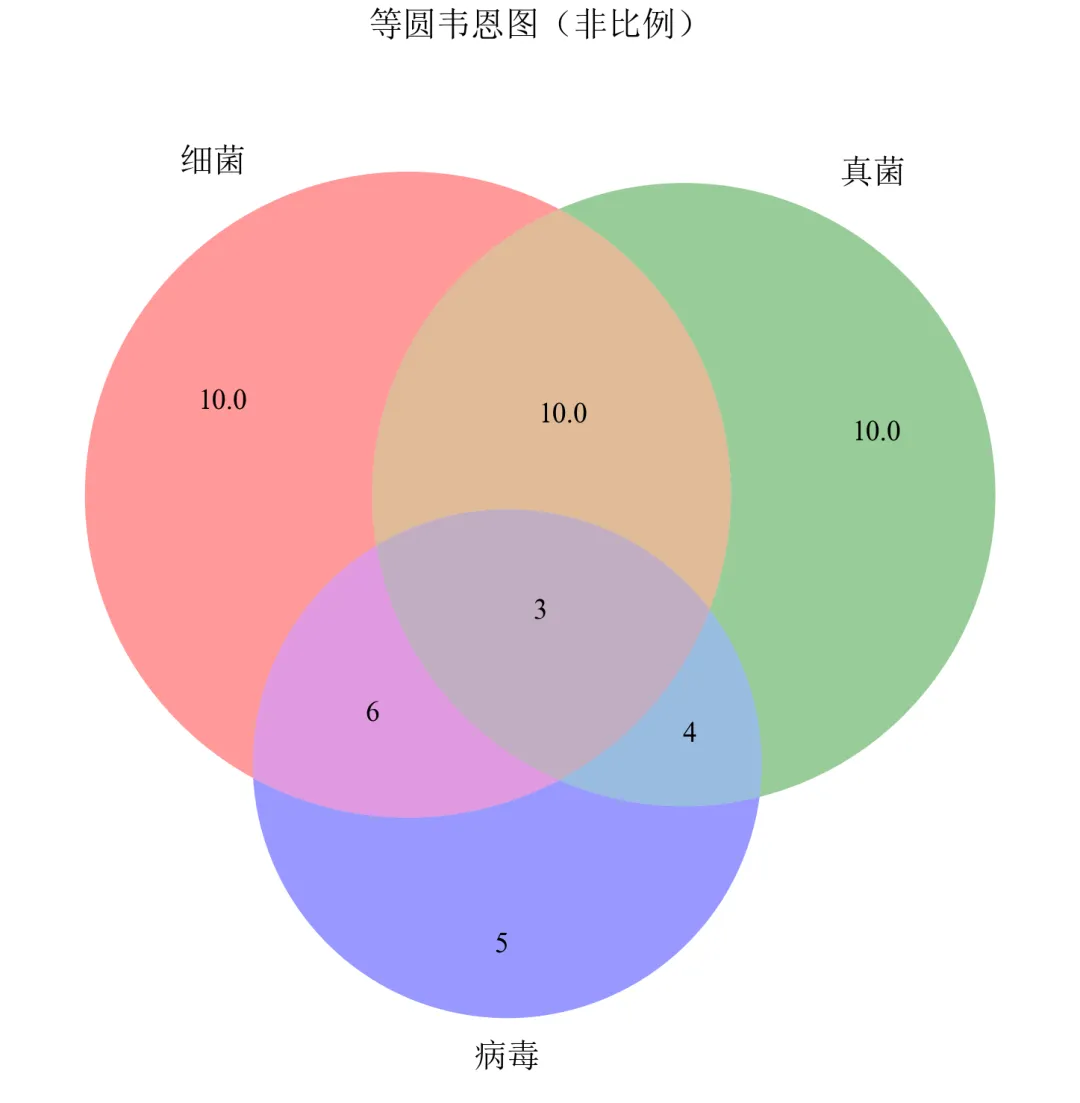
适用于强调集合交集关系、不关心基数比例的场景，如基因列表重叠展示。

进阶3：复杂韦恩图扩展——四元韦恩图

当集合数量时，传统韦恩图难以清晰展示，此处简要展示四元韦恩图方案。

import matplotlib.pyplot as pltfrom matplotlib_venn import venn3from matplotlib.patches import Circledefset_academic_style():    plt.rcParams['font.family'] = ['Times New Roman', 'SimSun']    plt.rcParams['font.size'] = 9    plt.rcParams['axes.unicode_minus'] = False    plt.rcParams['axes.linewidth'] = 1.0    plt.rcParams['xtick.major.width'] = 1.0    plt.rcParams['ytick.major.width'] = 1.0    plt.rcParams['xtick.major.size'] = 3.5    plt.rcParams['ytick.major.size'] = 3.5    plt.rcParams['xtick.direction'] = 'in'    plt.rcParams['ytick.direction'] = 'in'    plt.rcParams['legend.frameon'] = False    plt.rcParams['pdf.fonttype'] = 42    plt.rcParams['savefig.dpi'] = 300set_academic_style()# 创建图形fig, ax = plt.subplots(figsize=(8.0, 8.0))# 绘制三元韦恩图venn3(subsets=(10, 8, 12, 5, 6, 4, 3),      set_labels=('细菌', '真菌', '病毒'), ax=ax)# 手动添加第四个圆（古菌）circle4 = Circle((0, -0.6), 0.5,                 alpha=0.3, color='purple',                 edgecolor='black', linewidth=1.5)ax.add_patch(circle4)ax.text(0, -0.9, '古菌', fontsize=11, ha='center', va='center')ax.set_title('四元韦恩图（三元+手动添加）', fontsize=12, pad=20)plt.tight_layout()plt.show()fig.savefig('四元韦恩图_备选.pdf', bbox_inches='tight', pad_inches=0.05)fig.savefig('四元韦恩图_备选.png', bbox_inches='tight', pad_inches=0.05)

执行结果分析：

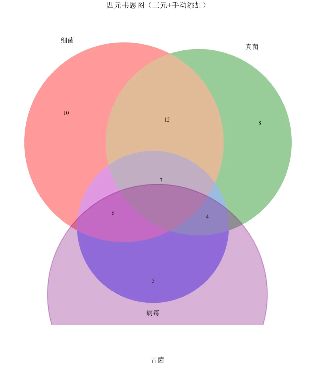
四元韦恩图由四个椭圆构成，阅读困难，一般不建议在论文中使用超过三元的韦恩图。

在撰写学术论文时，推荐三元以内用韦恩图。