《15节课Python绘图从入门到精通》5——直方图与核密度曲线的调参
- 2026-06-26 17:35:12
前置数据准备
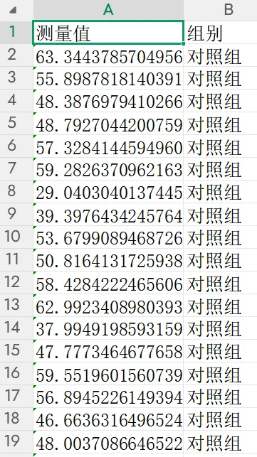
为保证所有程序可直接运行,先运行以下代码生成三组实验数据(对照组、处理组A、处理组B),每组包含一个连续型测量指标。
import pandas as pdimport numpy as npnp.random.seed(2024)n_per_group = 200# 对照组:正态分布,均值50,标准差8control = np.random.normal(50, 8, n_per_group)# 处理组A:右偏分布(对数正态),均值约55,标准差约12treatment_a = np.random.lognormal(mean=4.0, sigma=0.25, size=n_per_group) # 中位数约54.6# 处理组B:双峰分布(混合两个正态)treatment_b = np.concatenate([ np.random.normal(40, 5, int(n_per_group * 0.6)), np.random.normal(65, 6, int(n_per_group * 0.4))])# 构建长格式DataFrame,便于分组操作df_long = pd.DataFrame({'测量值': np.concatenate([control, treatment_a, treatment_b]),'组别': ['对照组'] * n_per_group + ['处理组A'] * n_per_group + ['处理组B'] * n_per_group})df_long.to_csv('三组实验数据.csv', index=False, encoding='utf-8-sig')print("数据生成完成:三组实验数据.csv(含'测量值'和'组别'两列)")print(f"每组样本量:{n_per_group}")执行结果如下(部分截图):
实操任务1:读取三组实验数据,绘制半透明堆叠直方图,对比分布形态差异
本任务从最基础的半透明直方图入手,逐步进阶到密度归一化、核密度曲线叠加、多面板排列及Seaborn快速绘制,符合顶刊数据分布对比规范。
基础版:半透明堆叠直方图(基本对比)
程序读取三组数据,在同一坐标系中绘制半透明直方图,通过颜色区分组别,直观对比分布形态。
import pandas as pdimport numpy as npimport matplotlib.pyplot as plt# 学术样式设置defset_academic_style(): plt.rcParams['font.family'] = ['Times New Roman', 'SimSun'] plt.rcParams['font.size'] = 9 plt.rcParams['axes.unicode_minus'] = False plt.rcParams['axes.linewidth'] = 1.0 plt.rcParams['xtick.major.width'] = 1.0 plt.rcParams['ytick.major.width'] = 1.0 plt.rcParams['xtick.major.size'] = 3.5 plt.rcParams['ytick.major.size'] = 3.5 plt.rcParams['xtick.direction'] = 'in' plt.rcParams['ytick.direction'] = 'in' plt.rcParams['legend.frameon'] = False plt.rcParams['pdf.fonttype'] = 42 plt.rcParams['savefig.dpi'] = 300set_academic_style()# 读取数据df = pd.read_csv('三组实验数据.csv')# 定义各组颜色(色盲友好配色)colors = {'对照组': '#4472C4', '处理组A': '#ED7D31', '处理组B': '#70AD47'}fig, ax = plt.subplots(figsize=(4.5, 3.5))# 分组绘制直方图,alpha控制透明度for group in df['组别'].unique(): subset = df[df['组别'] == group]['测量值'] ax.hist(subset, bins=25, alpha=0.5, color=colors[group], edgecolor='black', linewidth=0.3, label=group)ax.set_xlabel('测量值')ax.set_ylabel('频数')ax.legend(loc='upper right', fontsize=8)plt.tight_layout()plt.show()fig.savefig('半透明堆叠直方图_基础.pdf', bbox_inches='tight', pad_inches=0.05)fig.savefig('半透明堆叠直方图_基础.png', bbox_inches='tight', pad_inches=0.05)执行结果分析:
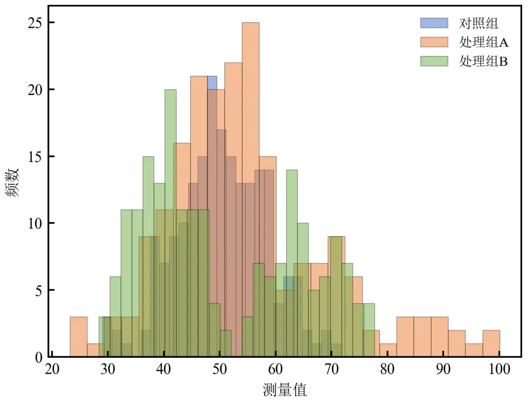
三组直方图重叠显示,半透明效果使重叠区域可见,便于比较分布中心、离散度和形态差异。
对照组呈对称分布,处理组A右偏,处理组B呈现双峰特征,直观展示组间异质性。
调整bins和alpha可优化视觉效果;alpha=0.5为常用透明度值。
进阶1:密度归一化直方图(纵轴为概率密度)
将直方图纵轴转换为概率密度,使各组面积均为1,消除样本量差异影响,便于比较分布形态。
import pandas as pdimport numpy as npimport matplotlib.pyplot as pltdefset_academic_style(): plt.rcParams['font.family'] = ['Times New Roman', 'SimSun'] plt.rcParams['font.size'] = 9 plt.rcParams['axes.unicode_minus'] = False plt.rcParams['axes.linewidth'] = 1.0 plt.rcParams['xtick.major.width'] = 1.0 plt.rcParams['ytick.major.width'] = 1.0 plt.rcParams['xtick.major.size'] = 3.5 plt.rcParams['ytick.major.size'] = 3.5 plt.rcParams['xtick.direction'] = 'in' plt.rcParams['ytick.direction'] = 'in' plt.rcParams['legend.frameon'] = False plt.rcParams['pdf.fonttype'] = 42 plt.rcParams['savefig.dpi'] = 300set_academic_style()df = pd.read_csv('三组实验数据.csv')colors = {'对照组': '#4472C4', '处理组A': '#ED7D31', '处理组B': '#70AD47'}fig, ax = plt.subplots(figsize=(4.5, 3.5))for group in df['组别'].unique(): subset = df[df['组别'] == group]['测量值'] ax.hist(subset, bins=25, density=True, alpha=0.5, color=colors[group], edgecolor='black', linewidth=0.3, label=group)ax.set_xlabel('测量值')ax.set_ylabel('概率密度')ax.legend(loc='upper right', fontsize=8)plt.tight_layout()plt.show()fig.savefig('密度归一化直方图.pdf', bbox_inches='tight', pad_inches=0.05)fig.savefig('密度归一化直方图.png', bbox_inches='tight', pad_inches=0.05)执行结果分析:
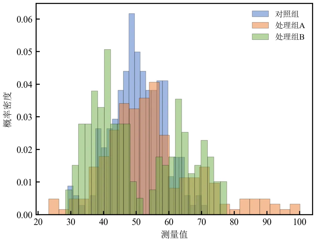
使用density=True使各组直方图面积归一化为1,纵轴变为概率密度,即使样本量不同也能公平比较分布形状。
处理组B的双峰在密度尺度下更明显,峰面积比例反映混合权重。
推荐在样本量不等或关注分布形态时使用。
进阶2:直方图叠加核密度曲线(平滑分布估计)
在直方图基础上叠加核密度估计(KDE)曲线,提供更平滑的分布形态参考。
import pandas as pdimport numpy as npimport matplotlib.pyplot as pltfrom scipy.stats import gaussian_kdedefset_academic_style(): plt.rcParams['font.family'] = ['Times New Roman', 'SimSun'] plt.rcParams['font.size'] = 9 plt.rcParams['axes.unicode_minus'] = False plt.rcParams['axes.linewidth'] = 1.0 plt.rcParams['xtick.major.width'] = 1.0 plt.rcParams['ytick.major.width'] = 1.0 plt.rcParams['xtick.major.size'] = 3.5 plt.rcParams['ytick.major.size'] = 3.5 plt.rcParams['xtick.direction'] = 'in' plt.rcParams['ytick.direction'] = 'in' plt.rcParams['legend.frameon'] = False plt.rcParams['pdf.fonttype'] = 42 plt.rcParams['savefig.dpi'] = 300set_academic_style()df = pd.read_csv('三组实验数据.csv')colors = {'对照组': '#4472C4', '处理组A': '#ED7D31', '处理组B': '#70AD47'}fig, ax = plt.subplots(figsize=(4.5, 3.5))for group in df['组别'].unique(): data = df[df['组别'] == group]['测量值'].values# 直方图(密度归一化) ax.hist(data, bins=25, density=True, alpha=0.4, color=colors[group], edgecolor='black', linewidth=0.3, label=f'{group} (直方图)')# KDE曲线 kde = gaussian_kde(data) x_grid = np.linspace(data.min(), data.max(), 200) ax.plot(x_grid, kde(x_grid), color=colors[group], linewidth=1.8, label=f'{group} (KDE)')# 为避免图例重复,可精简图例;此处保留完整图例便于理解handles, labels = ax.get_legend_handles_labels()# 仅保留KDE曲线图例(可选)ax.legend(handles[3:], labels[3:], loc='upper right', fontsize=8)ax.set_xlabel('测量值')ax.set_ylabel('概率密度')plt.tight_layout()plt.show()fig.savefig('直方图叠加KDE.pdf', bbox_inches='tight', pad_inches=0.05)fig.savefig('直方图叠加KDE.png', bbox_inches='tight', pad_inches=0.05)执行结果分析:
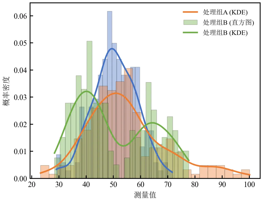
KDE曲线平滑展示分布形状,避免了直方图因分箱造成的人为锯齿。
处理组B的双峰在KDE中清晰呈现为两个峰,而直方图可能因分箱掩盖细节。
实际应用中,可仅保留KDE曲线图例,使图形更简洁。
进阶3:分面子图对比(各组分开展示)
当组间重叠严重时,将各组直方图分面绘制,并保持坐标轴范围一致,便于单独观察。
import pandas as pdimport numpy as npimport matplotlib.pyplot as pltdefset_academic_style(): plt.rcParams['font.family'] = ['Times New Roman', 'SimSun'] plt.rcParams['font.size'] = 9 plt.rcParams['axes.unicode_minus'] = False plt.rcParams['axes.linewidth'] = 1.0 plt.rcParams['xtick.major.width'] = 1.0 plt.rcParams['ytick.major.width'] = 1.0 plt.rcParams['xtick.major.size'] = 3.5 plt.rcParams['ytick.major.size'] = 3.5 plt.rcParams['xtick.direction'] = 'in' plt.rcParams['ytick.direction'] = 'in' plt.rcParams['legend.frameon'] = False plt.rcParams['pdf.fonttype'] = 42 plt.rcParams['savefig.dpi'] = 300set_academic_style()df = pd.read_csv('三组实验数据.csv')groups = df['组别'].unique()colors = {'对照组': '#4472C4', '处理组A': '#ED7D31', '处理组B': '#70AD47'}fig, axes = plt.subplots(1, 3, figsize=(9.0, 3.2), sharex=True, sharey=True)# 确定全局x轴范围x_min = df['测量值'].min() * 0.95x_max = df['测量值'].max() * 1.05for ax, group in zip(axes, groups): data = df[df['组别'] == group]['测量值'] ax.hist(data, bins=25, density=True, alpha=0.7, color=colors[group], edgecolor='black', linewidth=0.3) ax.set_title(group, fontsize=10) ax.set_xlabel('测量值') ax.set_ylabel('概率密度') ax.set_xlim(x_min, x_max)plt.tight_layout()plt.show()fig.savefig('分面直方图对比.pdf', bbox_inches='tight', pad_inches=0.05)fig.savefig('分面直方图对比.png', bbox_inches='tight', pad_inches=0.05)执行结果分析:
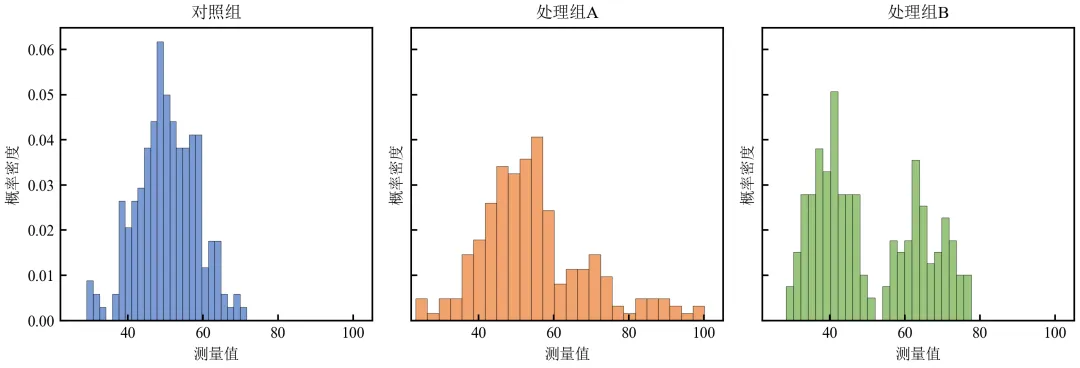
分面显示消除了重叠干扰,各组的分布特征一目了然。
共享坐标轴使组间可直接比较位置和离散度。
适用于组间分布差异显著且需要独立展示的情况。
进阶4:Seaborn快速绘制
利用Seaborn库简化绘图代码,可以一行代码实现分组直方图+KDE,同时保持出版级美观。
import pandas as pdimport matplotlib.pyplot as pltimport seaborn as snsdefset_academic_style(): plt.rcParams['font.family'] = ['Times New Roman', 'SimSun'] plt.rcParams['font.size'] = 9 plt.rcParams['axes.unicode_minus'] = False plt.rcParams['axes.linewidth'] = 1.0 plt.rcParams['xtick.major.width'] = 1.0 plt.rcParams['ytick.major.width'] = 1.0 plt.rcParams['xtick.major.size'] = 3.5 plt.rcParams['ytick.major.size'] = 3.5 plt.rcParams['xtick.direction'] = 'in' plt.rcParams['ytick.direction'] = 'in' plt.rcParams['legend.frameon'] = False plt.rcParams['pdf.fonttype'] = 42 plt.rcParams['savefig.dpi'] = 300set_academic_style()df = pd.read_csv('三组实验数据.csv')fig, ax = plt.subplots(figsize=(4.5, 3.5))# 使用seaborn的histplot,设置元素类型和透明度sns.histplot(data=df, x='测量值', hue='组别', bins=25, alpha=0.5, kde=True, palette=['#4472C4', '#ED7D31', '#70AD47'], edgecolor='black', linewidth=0.3, ax=ax)ax.set_xlabel('测量值')ax.set_ylabel('频数')# Seaborn图例默认有边框,需手动去除legend = ax.get_legend()if legend: legend.set_frame_on(False)plt.tight_layout()plt.show()fig.savefig('Seaborn分组直方图_KDE.pdf', bbox_inches='tight', pad_inches=0.05)fig.savefig('Seaborn分组直方图_KDE.png', bbox_inches='tight', pad_inches=0.05)执行结果分析:
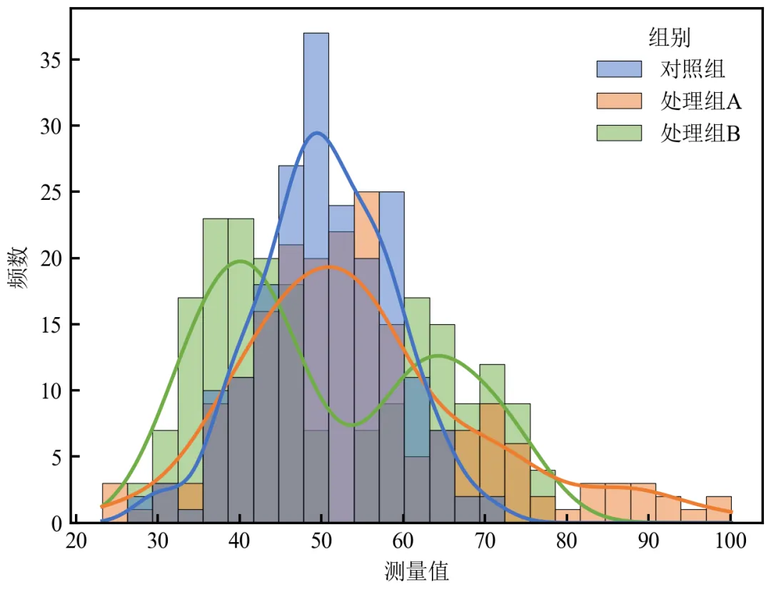
Seaborn一行代码实现分组直方图叠加KDE,显著减少代码量。
内置美观配色和自动图例,适合快速探索性分析。
可通过kde=True直接添加密度曲线,无需手动计算。
实操任务2:调整bins参数
直方图的bins(分箱数)选择对分布形态的呈现至关重要。本任务通过可视化对比不同bins的效果,并介绍几种自动确定最优bins的统计方法。
基础版:bins参数对比网格(欠平滑 → 过平滑)
使用同一组数据,绘制不同bins值的直方图,直观展示bins对分布解读的影响。
import pandas as pdimport numpy as npimport matplotlib.pyplot as pltdefset_academic_style(): plt.rcParams['font.family'] = ['Times New Roman', 'SimSun'] plt.rcParams['font.size'] = 9 plt.rcParams['axes.unicode_minus'] = False plt.rcParams['axes.linewidth'] = 1.0 plt.rcParams['xtick.major.width'] = 1.0 plt.rcParams['ytick.major.width'] = 1.0 plt.rcParams['xtick.major.size'] = 3.5 plt.rcParams['ytick.major.size'] = 3.5 plt.rcParams['xtick.direction'] = 'in' plt.rcParams['ytick.direction'] = 'in' plt.rcParams['legend.frameon'] = False plt.rcParams['pdf.fonttype'] = 42 plt.rcParams['savefig.dpi'] = 300set_academic_style()df = pd.read_csv('三组实验数据.csv')# 使用对照组数据作为示例data = df[df['组别'] == '对照组']['测量值'].values# 定义不同bins值bins_list = [5, 15, 30, 60]fig, axes = plt.subplots(2, 2, figsize=(6.5, 5.0))axes = axes.flatten()for ax, bins in zip(axes, bins_list): ax.hist(data, bins=bins, color='#4472C4', alpha=0.7, edgecolor='black', linewidth=0.3) ax.set_title(f'bins = {bins}', fontsize=10) ax.set_xlabel('测量值') ax.set_ylabel('频数')# 添加描述标签if bins == 5: ax.text(0.95, 0.95, '欠平滑', transform=ax.transAxes, ha='right', va='top', bbox=dict(boxstyle='round', facecolor='white', alpha=0.8))elif bins == 15: ax.text(0.95, 0.95, '适中', transform=ax.transAxes, ha='right', va='top', bbox=dict(boxstyle='round', facecolor='white', alpha=0.8))elif bins == 60: ax.text(0.95, 0.95, '过平滑', transform=ax.transAxes, ha='right', va='top', bbox=dict(boxstyle='round', facecolor='white', alpha=0.8))plt.tight_layout()plt.show()fig.savefig('bins参数对比网格.pdf', bbox_inches='tight', pad_inches=0.05)fig.savefig('bins参数对比网格.png', bbox_inches='tight', pad_inches=0.05)执行结果分析:
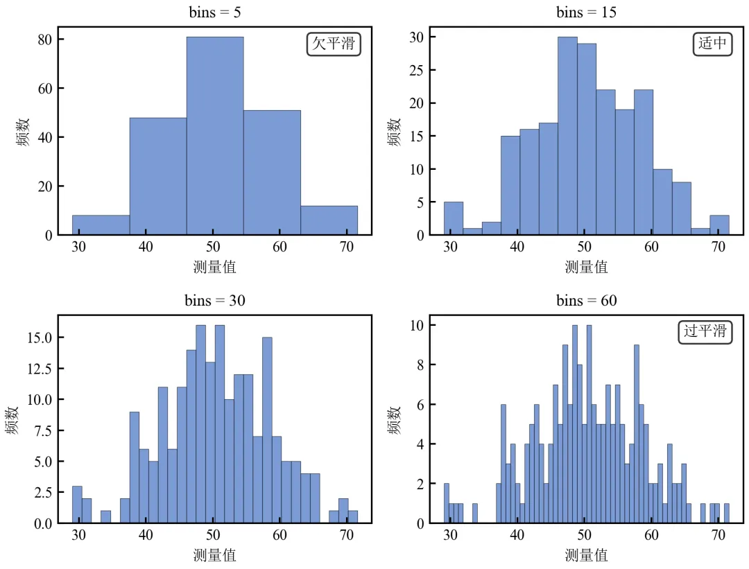
bins=5:分箱过宽,丢失分布细节,呈“欠平滑”状态。
bins=15:清晰展示分布的单峰对称形态,为“适中”选择。
bins=30~60:分箱过细,出现大量空箱和噪声,呈“过平滑/过拟合”状态,干扰分布判断。
最优bins通常在15~30之间,取决于样本量和数据范围。
进阶1:自动计算最优bins(Sturges、Scott、Freedman-Diaconis规则)
使用统计学公式自动推荐bins数,并可视化对比。
import pandas as pdimport numpy as npimport matplotlib.pyplot as pltdefset_academic_style(): plt.rcParams['font.family'] = ['Times New Roman', 'SimSun'] plt.rcParams['font.size'] = 9 plt.rcParams['axes.unicode_minus'] = False plt.rcParams['axes.linewidth'] = 1.0 plt.rcParams['xtick.major.width'] = 1.0 plt.rcParams['ytick.major.width'] = 1.0 plt.rcParams['xtick.major.size'] = 3.5 plt.rcParams['ytick.major.size'] = 3.5 plt.rcParams['xtick.direction'] = 'in' plt.rcParams['ytick.direction'] = 'in' plt.rcParams['legend.frameon'] = False plt.rcParams['pdf.fonttype'] = 42 plt.rcParams['savefig.dpi'] = 300set_academic_style()df = pd.read_csv('三组实验数据.csv')data = df[df['组别'] == '对照组']['测量值'].valuesn = len(data)# 计算三种规则推荐的bins数# Sturges: k = ceil(log2(n) + 1)bins_sturges = int(np.ceil(np.log2(n) + 1))# Scott: bin_width = 3.5 * std / n^(1/3) → bins = range / widthbin_width_scott = 3.5 * np.std(data) / (n ** (1/3))bins_scott = int(np.ceil((data.max() - data.min()) / bin_width_scott))# Freedman-Diaconis: bin_width = 2 * IQR / n^(1/3)iqr = np.percentile(data, 75) - np.percentile(data, 25)bin_width_fd = 2 * iqr / (n ** (1/3))bins_fd = int(np.ceil((data.max() - data.min()) / bin_width_fd))print(f"Sturges推荐bins: {bins_sturges}")print(f"Scott推荐bins: {bins_scott}")print(f"Freedman-Diaconis推荐bins: {bins_fd}")# 绘制三个推荐bins的直方图对比fig, axes = plt.subplots(1, 3, figsize=(9.0, 3.0))bins_dict = {'Sturges': bins_sturges, 'Scott': bins_scott, 'F-D': bins_fd}for ax, (name, b) in zip(axes, bins_dict.items()): ax.hist(data, bins=b, color='#4472C4', alpha=0.7, edgecolor='black', linewidth=0.3) ax.set_title(f'{name} (bins={b})') ax.set_xlabel('测量值') ax.set_ylabel('频数')plt.tight_layout()plt.show()fig.savefig('自动bins规则对比.pdf', bbox_inches='tight', pad_inches=0.05)fig.savefig('自动bins规则对比.png', bbox_inches='tight', pad_inches=0.05)执行结果分析:
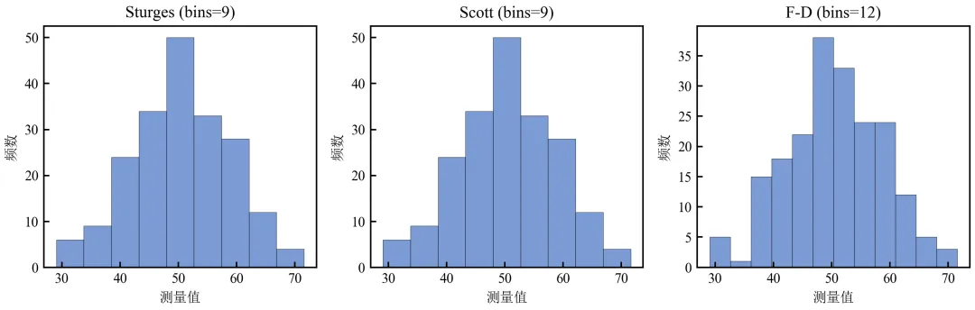
Sturges规则适用于正态分布小样本,n=200时推荐约9 bins,略显保守。
Scott规则基于标准差,对正态数据表现良好,推荐约9 bins。
Freedman-Diaconis规则基于IQR,对异常值鲁棒,推荐约12 bins。
实际应用中,可将这些值作为起点,结合领域知识微调。
进阶2:分组数据的最优bins对比(各组独立确定)
不同组数据分布差异大时,可为每组独立计算最优bins并绘制。
import pandas as pdimport numpy as npimport matplotlib.pyplot as pltdefset_academic_style(): plt.rcParams['font.family'] = ['Times New Roman', 'SimSun'] plt.rcParams['font.size'] = 9 plt.rcParams['axes.unicode_minus'] = False plt.rcParams['axes.linewidth'] = 1.0 plt.rcParams['xtick.major.width'] = 1.0 plt.rcParams['ytick.major.width'] = 1.0 plt.rcParams['xtick.major.size'] = 3.5 plt.rcParams['ytick.major.size'] = 3.5 plt.rcParams['xtick.direction'] = 'in' plt.rcParams['ytick.direction'] = 'in' plt.rcParams['legend.frameon'] = False plt.rcParams['pdf.fonttype'] = 42 plt.rcParams['savefig.dpi'] = 300set_academic_style()df = pd.read_csv('三组实验数据.csv')groups = df['组别'].unique()colors = {'对照组': '#4472C4', '处理组A': '#ED7D31', '处理组B': '#70AD47'}fig, axes = plt.subplots(1, 3, figsize=(9.0, 3.2), sharex=True, sharey=False)for ax, group in zip(axes, groups): data = df[df['组别'] == group]['测量值'].values n = len(data)# 使用Freedman-Diaconis规则计算bins iqr = np.percentile(data, 75) - np.percentile(data, 25) bin_width = 2 * iqr / (n ** (1/3)) bins = int(np.ceil((data.max() - data.min()) / bin_width)) ax.hist(data, bins=bins, density=True, color=colors[group], alpha=0.7, edgecolor='black', linewidth=0.3) ax.set_title(f'{group} (bins={bins})') ax.set_xlabel('测量值') ax.set_ylabel('概率密度')plt.tight_layout()plt.show()fig.savefig('分组最优bins直方图.pdf', bbox_inches='tight', pad_inches=0.05)fig.savefig('分组最优bins直方图.png', bbox_inches='tight', pad_inches=0.05)执行结果分析:
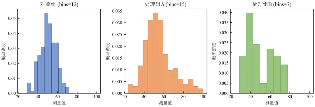
处理组A(右偏)和B(双峰)所需bins数与对照组不同,独立确定能更好地揭示分布特征。
进阶3:直方图与核密度曲线联合确定最优bins(视觉校准)
通过叠加核密度曲线,评估直方图bins是否与平滑分布估计一致。
import pandas as pdimport numpy as npimport matplotlib.pyplot as pltfrom scipy.stats import gaussian_kdedefset_academic_style(): plt.rcParams['font.family'] = ['Times New Roman', 'SimSun'] plt.rcParams['font.size'] = 9 plt.rcParams['axes.unicode_minus'] = False plt.rcParams['axes.linewidth'] = 1.0 plt.rcParams['xtick.major.width'] = 1.0 plt.rcParams['ytick.major.width'] = 1.0 plt.rcParams['xtick.major.size'] = 3.5 plt.rcParams['ytick.major.size'] = 3.5 plt.rcParams['xtick.direction'] = 'in' plt.rcParams['ytick.direction'] = 'in' plt.rcParams['legend.frameon'] = False plt.rcParams['pdf.fonttype'] = 42 plt.rcParams['savefig.dpi'] = 300set_academic_style()df = pd.read_csv('三组实验数据.csv')data = df[df['组别'] == '对照组']['测量值'].valueskde = gaussian_kde(data)x_grid = np.linspace(data.min(), data.max(), 200)bins_list = [5, 15, 30]fig, axes = plt.subplots(1, 3, figsize=(9.0, 3.0))for ax, bins in zip(axes, bins_list): ax.hist(data, bins=bins, density=True, color='#4472C4', alpha=0.6, edgecolor='black', linewidth=0.3, label=f'bins={bins}') ax.plot(x_grid, kde(x_grid), color='#C00000', linewidth=1.8, label='KDE') ax.set_xlabel('测量值') ax.set_ylabel('概率密度') ax.legend(loc='upper right', fontsize=8)plt.tight_layout()plt.show()fig.savefig('bins与KDE联合校准.pdf', bbox_inches='tight', pad_inches=0.05)fig.savefig('bins与KDE联合校准.png', bbox_inches='tight', pad_inches=0.05)执行结果分析:
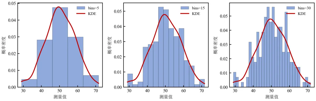
KDE曲线作为“真值”参考,bins=15时直方图与KDE吻合最佳。
bins=5过于平滑,丢失峰部细节;bins=30出现噪声波动,与KDE偏离。
此方法可帮助研究者可视化地确定最优bins。
实操任务3:绘制累积分布函数曲线,对比对照组与处理组在各百分位数上的差异
累积分布函数(CDF)能清晰展示数据的百分位数、分布形状及组间差异,无需分箱,不受主观参数影响。本任务从基础ECDF绘制进阶到多组对比、KS检验标注及对数坐标。
基础版:两组数据的ECDF曲线对比
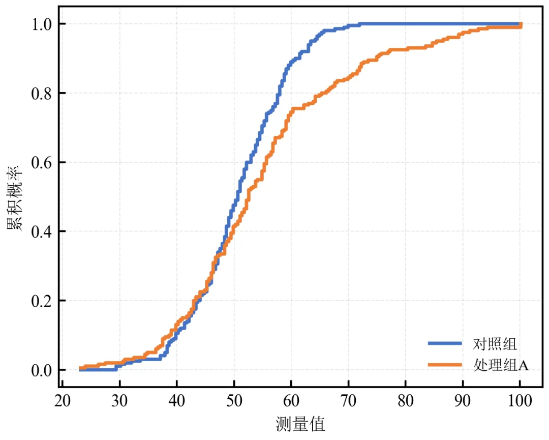
绘制对照组与处理组A的经验累积分布函数,直观比较分布位置和形状。
import pandas as pdimport numpy as npimport matplotlib.pyplot as pltdefset_academic_style(): plt.rcParams['font.family'] = ['Times New Roman', 'SimSun'] plt.rcParams['font.size'] = 9 plt.rcParams['axes.unicode_minus'] = False plt.rcParams['axes.linewidth'] = 1.0 plt.rcParams['xtick.major.width'] = 1.0 plt.rcParams['ytick.major.width'] = 1.0 plt.rcParams['xtick.major.size'] = 3.5 plt.rcParams['ytick.major.size'] = 3.5 plt.rcParams['xtick.direction'] = 'in' plt.rcParams['ytick.direction'] = 'in' plt.rcParams['legend.frameon'] = False plt.rcParams['pdf.fonttype'] = 42 plt.rcParams['savefig.dpi'] = 300set_academic_style()df = pd.read_csv('三组实验数据.csv')control = df[df['组别'] == '对照组']['测量值'].valuestreat_a = df[df['组别'] == '处理组A']['测量值'].values# 计算ECDFdefecdf(data): x = np.sort(data) y = np.arange(1, len(data)+1) / len(data)return x, yx_ctrl, y_ctrl = ecdf(control)x_a, y_a = ecdf(treat_a)fig, ax = plt.subplots(figsize=(4.2, 3.4))ax.step(x_ctrl, y_ctrl, where='post', color='#4472C4', linewidth=1.8, label='对照组')ax.step(x_a, y_a, where='post', color='#ED7D31', linewidth=1.8, label='处理组A')ax.set_xlabel('测量值')ax.set_ylabel('累积概率')ax.legend(loc='lower right', fontsize=8)ax.grid(alpha=0.3, linestyle='--', linewidth=0.5)plt.tight_layout()plt.show()fig.savefig('ECDF两组对比.pdf', bbox_inches='tight', pad_inches=0.05)fig.savefig('ECDF两组对比.png', bbox_inches='tight', pad_inches=0.05)执行结果分析:
阶梯状ECDF曲线显示数据的累积比例,处理组A曲线整体右移,表明其值普遍高于对照组。
曲线斜率反映概率密度:陡峭处对应高密度区域,平缓处对应低密度区域。
可轻松读取任意分位数,如中位数(y=0.5对应的x值)。
进阶1:标注关键百分位数(中位数、四分位数)
在ECDF曲线上添加水平线和垂直线,突出显示特定百分位数。
import pandas as pdimport numpy as npimport matplotlib.pyplot as pltdefset_academic_style(): plt.rcParams['font.family'] = ['Times New Roman', 'SimSun'] plt.rcParams['font.size'] = 9 plt.rcParams['axes.unicode_minus'] = False plt.rcParams['axes.linewidth'] = 1.0 plt.rcParams['xtick.major.width'] = 1.0 plt.rcParams['ytick.major.width'] = 1.0 plt.rcParams['xtick.major.size'] = 3.5 plt.rcParams['ytick.major.size'] = 3.5 plt.rcParams['xtick.direction'] = 'in' plt.rcParams['ytick.direction'] = 'in' plt.rcParams['legend.frameon'] = False plt.rcParams['pdf.fonttype'] = 42 plt.rcParams['savefig.dpi'] = 300set_academic_style()df = pd.read_csv('三组实验数据.csv')control = df[df['组别'] == '对照组']['测量值'].valuestreat_a = df[df['组别'] == '处理组A']['测量值'].valuesdefecdf(data): x = np.sort(data) y = np.arange(1, len(data)+1) / len(data)return x, yx_ctrl, y_ctrl = ecdf(control)x_a, y_a = ecdf(treat_a)fig, ax = plt.subplots(figsize=(4.5, 3.5))ax.step(x_ctrl, y_ctrl, where='post', color='#4472C4', linewidth=1.8, label='对照组')ax.step(x_a, y_a, where='post', color='#ED7D31', linewidth=1.8, label='处理组A')# 绘制水平参考线(只画一次)ax.axhline(y=0.5, color='gray', linestyle=':', linewidth=0.8, alpha=0.6)ax.axhline(y=0.25, color='gray', linestyle=':', linewidth=0.5, alpha=0.4)ax.axhline(y=0.75, color='gray', linestyle=':', linewidth=0.5, alpha=0.4)# 标注中位数和四分位数# 对照组median_ctrl = np.median(control)q1_ctrl = np.percentile(control, 25)q3_ctrl = np.percentile(control, 75)ax.axvline(x=median_ctrl, color='#4472C4', linestyle='--', linewidth=0.8, alpha=0.7)ax.axvline(x=q1_ctrl, color='#4472C4', linestyle=':', linewidth=0.6, alpha=0.5)ax.axvline(x=q3_ctrl, color='#4472C4', linestyle=':', linewidth=0.6, alpha=0.5)ax.text(median_ctrl, 0.53, f'中位数={median_ctrl:.1f}', color='#4472C4', fontsize=7, ha='center')ax.text(q1_ctrl, 0.28, f'Q1={q1_ctrl:.1f}', color='#4472C4', fontsize=7, ha='center')ax.text(q3_ctrl, 0.78, f'Q3={q3_ctrl:.1f}', color='#4472C4', fontsize=7, ha='center')# 处理组Amedian_a = np.median(treat_a)q1_a = np.percentile(treat_a, 25)q3_a = np.percentile(treat_a, 75)ax.axvline(x=median_a, color='#ED7D31', linestyle='--', linewidth=0.8, alpha=0.7)ax.axvline(x=q1_a, color='#ED7D31', linestyle=':', linewidth=0.6, alpha=0.5)ax.axvline(x=q3_a, color='#ED7D31', linestyle=':', linewidth=0.6, alpha=0.5)ax.text(median_a, 0.47, f'中位数={median_a:.1f}', color='#ED7D31', fontsize=7, ha='center')ax.text(q1_a, 0.22, f'Q1={q1_a:.1f}', color='#ED7D31', fontsize=7, ha='center')ax.text(q3_a, 0.72, f'Q3={q3_a:.1f}', color='#ED7D31', fontsize=7, ha='center')ax.set_xlabel('测量值')ax.set_ylabel('累积概率')ax.legend(loc='lower right', fontsize=8)ax.grid(alpha=0.3, linestyle='--', linewidth=0.5)plt.tight_layout()plt.show()fig.savefig('ECDF标注百分位数.pdf', bbox_inches='tight', pad_inches=0.05)fig.savefig('ECDF标注百分位数.png', bbox_inches='tight', pad_inches=0.05)执行结果分析:
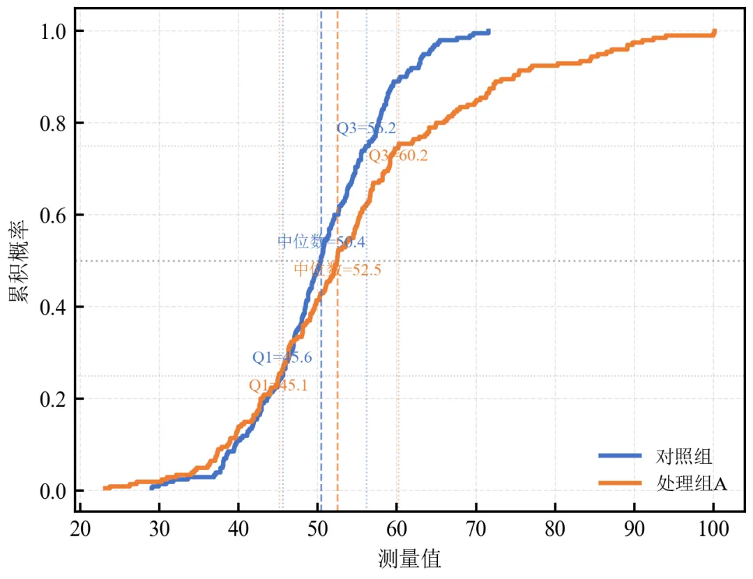
灰色水平线标记累积概率0.25、0.5、0.75,垂直虚线标出各组中位数位置。
处理组A中位数(52.5)明显高于对照组(50.4)
此类标注使百分位数对比定量化,适合报告关键统计量。
进阶2:多组ECDF对比 + Kolmogorov-Smirnov检验结果标注
计算两组间KS统计量及p值,并标注在图上,量化分布差异显著性。
import pandas as pdimport numpy as npimport matplotlib.pyplot as pltfrom scipy.stats import ks_2sampdefset_academic_style(): plt.rcParams['font.family'] = ['Times New Roman', 'SimSun'] plt.rcParams['font.size'] = 9 plt.rcParams['axes.unicode_minus'] = False plt.rcParams['axes.linewidth'] = 1.0 plt.rcParams['xtick.major.width'] = 1.0 plt.rcParams['ytick.major.width'] = 1.0 plt.rcParams['xtick.major.size'] = 3.5 plt.rcParams['ytick.major.size'] = 3.5 plt.rcParams['xtick.direction'] = 'in' plt.rcParams['ytick.direction'] = 'in' plt.rcParams['legend.frameon'] = False plt.rcParams['pdf.fonttype'] = 42 plt.rcParams['savefig.dpi'] = 300set_academic_style()df = pd.read_csv('三组实验数据.csv')groups = ['对照组', '处理组A', '处理组B']colors = ['#4472C4', '#ED7D31', '#70AD47']defecdf(data): x = np.sort(data) y = np.arange(1, len(data)+1) / len(data)return x, yfig, ax = plt.subplots(figsize=(4.8, 3.6))for group, color in zip(groups, colors): data = df[df['组别'] == group]['测量值'].values x_ecdf, y_ecdf = ecdf(data) ax.step(x_ecdf, y_ecdf, where='post', color=color, linewidth=1.8, label=group)# 对照组 vs 处理组A KS检验ctrl = df[df['组别'] == '对照组']['测量值'].valuestreat_a = df[df['组别'] == '处理组A']['测量值'].valuesks_stat, p_value = ks_2samp(ctrl, treat_a)ax.text(0.05, 0.85, f'KS检验 (对照 vs 处理A):\nD = {ks_stat:.3f}, p = {p_value:.3e}', transform=ax.transAxes, fontsize=8, bbox=dict(boxstyle='round', facecolor='white', alpha=0.8))ax.set_xlabel('测量值')ax.set_ylabel('累积概率')ax.legend(loc='lower right', fontsize=8)ax.grid(alpha=0.3, linestyle='--', linewidth=0.5)plt.tight_layout()plt.show()fig.savefig('ECDF多组_KS检验.pdf', bbox_inches='tight', pad_inches=0.05)fig.savefig('ECDF多组_KS检验.png', bbox_inches='tight', pad_inches=0.05)执行结果分析:
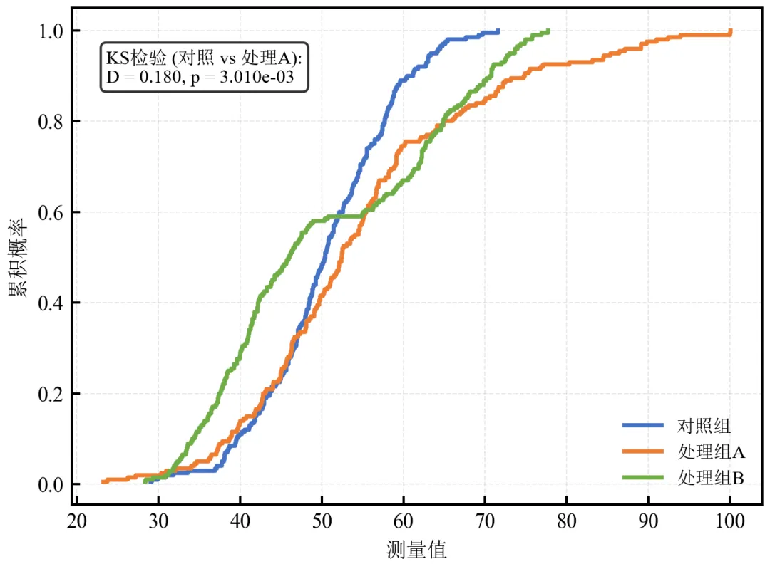
三组ECDF曲线清晰展示分布差异,处理组B双峰导致曲线在中段出现平台。
KS检验p值极小,表明对照组与处理组A分布差异极显著。
在学术论文中,ECDF配合KS检验是严谨的分布对比方法。
进阶3:使用statsmodels的ECDF绘图函数(简化代码)
statsmodels库提供ECDF类,可直接生成ECDF对象并绘图,减少手动编码。
import pandas as pdimport numpy as npimport matplotlib.pyplot as pltimport statsmodels.api as smdefset_academic_style(): plt.rcParams['font.family'] = ['Times New Roman', 'SimSun'] plt.rcParams['font.size'] = 9 plt.rcParams['axes.unicode_minus'] = False plt.rcParams['axes.linewidth'] = 1.0 plt.rcParams['xtick.major.width'] = 1.0 plt.rcParams['ytick.major.width'] = 1.0 plt.rcParams['xtick.major.size'] = 3.5 plt.rcParams['ytick.major.size'] = 3.5 plt.rcParams['xtick.direction'] = 'in' plt.rcParams['ytick.direction'] = 'in' plt.rcParams['legend.frameon'] = False plt.rcParams['pdf.fonttype'] = 42 plt.rcParams['savefig.dpi'] = 300set_academic_style()df = pd.read_csv('三组实验数据.csv')control = df[df['组别'] == '对照组']['测量值'].valuestreat_a = df[df['组别'] == '处理组A']['测量值'].valuesecdf_ctrl = sm.distributions.ECDF(control)ecdf_a = sm.distributions.ECDF(treat_a)fig, ax = plt.subplots(figsize=(4.2, 3.4))x_plot = np.linspace(df['测量值'].min(), df['测量值'].max(), 200)ax.step(x_plot, ecdf_ctrl(x_plot), where='post', color='#4472C4', linewidth=1.8, label='对照组')ax.step(x_plot, ecdf_a(x_plot), where='post', color='#ED7D31', linewidth=1.8, label='处理组A')ax.set_xlabel('测量值')ax.set_ylabel('累积概率')ax.legend(loc='lower right', fontsize=8)ax.grid(alpha=0.3, linestyle='--', linewidth=0.5)plt.tight_layout()plt.show()fig.savefig('ECDF_statsmodels.pdf', bbox_inches='tight', pad_inches=0.05)fig.savefig('ECDF_statsmodels.png', bbox_inches='tight', pad_inches=0.05)执行结果分析:
statsmodels的ECDF类封装了计算逻辑,调用ecdf(x)即可获得累积概率,代码更简洁。
适合快速生成ECDF图,尤其在与statsmodels其他统计功能联用时。
进阶4:对数坐标轴下的ECDF(处理长尾数据)
当数据跨越多个数量级时,将x轴转换为对数坐标,可更好展示低值区域的分布细节。
import pandas as pdimport numpy as npimport matplotlib.pyplot as pltdefset_academic_style(): plt.rcParams['font.family'] = ['Times New Roman', 'SimSun'] plt.rcParams['font.size'] = 9 plt.rcParams['axes.unicode_minus'] = False plt.rcParams['axes.linewidth'] = 1.0 plt.rcParams['xtick.major.width'] = 1.0 plt.rcParams['ytick.major.width'] = 1.0 plt.rcParams['xtick.major.size'] = 3.5 plt.rcParams['ytick.major.size'] = 3.5 plt.rcParams['xtick.direction'] = 'in' plt.rcParams['ytick.direction'] = 'in' plt.rcParams['legend.frameon'] = False plt.rcParams['pdf.fonttype'] = 42 plt.rcParams['savefig.dpi'] = 300set_academic_style()# 模拟长尾数据(处理组A本身是对数正态,已具长尾;为演示更明显,可生成新数据)np.random.seed(2024)long_tail = np.random.lognormal(mean=4.0, sigma=0.8, size=500) # 更明显的长尾normal_data = np.random.normal(50, 8, 500)defecdf(data): x = np.sort(data) y = np.arange(1, len(data)+1) / len(data)return x, yx_lt, y_lt = ecdf(long_tail)x_norm, y_norm = ecdf(normal_data)fig, (ax1, ax2) = plt.subplots(1, 2, figsize=(7.0, 3.2))# 线性坐标ax1.step(x_lt, y_lt, where='post', color='#ED7D31', linewidth=1.8, label='长尾分布')ax1.step(x_norm, y_norm, where='post', color='#4472C4', linewidth=1.8, label='正态分布')ax1.set_xlabel('测量值')ax1.set_ylabel('累积概率')ax1.legend(loc='lower right', fontsize=8)ax1.grid(alpha=0.3, linestyle='--', linewidth=0.5)ax1.set_title('线性坐标')# 对数坐标ax2.step(x_lt, y_lt, where='post', color='#ED7D31', linewidth=1.8, label='长尾分布')ax2.step(x_norm, y_norm, where='post', color='#4472C4', linewidth=1.8, label='正态分布')ax2.set_xscale('log')ax2.set_xlabel('测量值 (对数坐标)')ax2.set_ylabel('累积概率')ax2.legend(loc='lower right', fontsize=8)ax2.grid(alpha=0.3, linestyle='--', linewidth=0.5)ax2.set_title('对数坐标')plt.tight_layout()plt.show()fig.savefig('ECDF对数坐标.pdf', bbox_inches='tight', pad_inches=0.05)fig.savefig('ECDF对数坐标.png', bbox_inches='tight', pad_inches=0.05)执行结果分析:
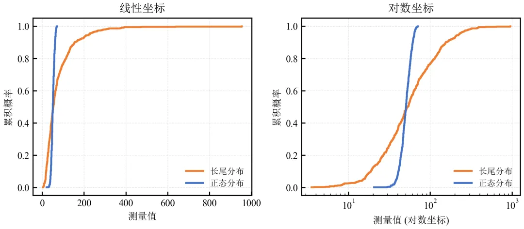
线性坐标下,长尾分布的高值区域被压缩,低值区域细节难以辨认。
对数坐标拉伸低值区域,清晰展示长尾分布的上升形态,便于比较不同分布的低百分位数。
适用于收入、基因表达量、粒径等对数正态分布数据。
实操任务4:绘制小提琴图
小提琴图结合了箱线图和核密度估计,既能展示分布形态,又能显示关键统计量。本任务从基础绘制进阶到自定义美化、分组对比及散点叠加。
基础版:Seaborn快速绘制带内嵌箱线图的小提琴图
Seaborn的violinplot函数可直接在内部绘制微型箱线图,参数inner='box'即可实现。
import pandas as pdimport matplotlib.pyplot as pltimport seaborn as snsdefset_academic_style(): plt.rcParams['font.family'] = ['Times New Roman', 'SimSun'] plt.rcParams['font.size'] = 9 plt.rcParams['axes.unicode_minus'] = False plt.rcParams['axes.linewidth'] = 1.0 plt.rcParams['xtick.major.width'] = 1.0 plt.rcParams['ytick.major.width'] = 1.0 plt.rcParams['xtick.major.size'] = 3.5 plt.rcParams['ytick.major.size'] = 3.5 plt.rcParams['xtick.direction'] = 'in' plt.rcParams['ytick.direction'] = 'in' plt.rcParams['legend.frameon'] = False plt.rcParams['pdf.fonttype'] = 42 plt.rcParams['savefig.dpi'] = 300set_academic_style()df = pd.read_csv('三组实验数据.csv')fig, ax = plt.subplots(figsize=(4.5, 4.0))sns.violinplot(data=df, x='组别', y='测量值', inner='box', palette=['#4472C4', '#ED7D31', '#70AD47'], linewidth=0.8, ax=ax)ax.set_xlabel('组别')ax.set_ylabel('测量值')# 去除上、右 spinessns.despine()plt.tight_layout()plt.show()fig.savefig('小提琴图_基础.pdf', bbox_inches='tight', pad_inches=0.05)fig.savefig('小提琴图_基础.png', bbox_inches='tight', pad_inches=0.05)执行结果分析:
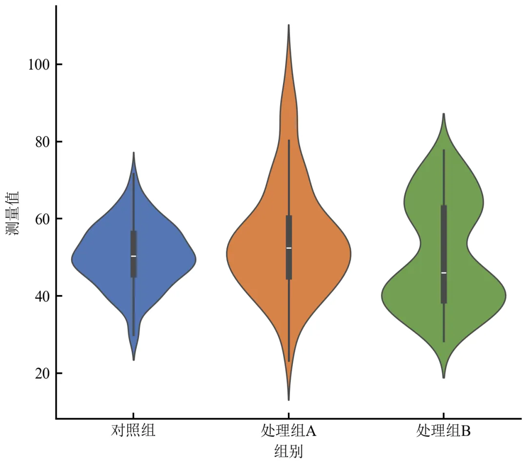
小提琴宽度反映概率密度,处理组A右偏、处理组B双峰形态一目了然。
内部白色箱线图显示中位数(白点)、四分位距(粗黑线)及须线范围。
Seaborn自动处理分组与配色,代码极简。
进阶1:自定义小提琴图细节(线宽、颜色、透明度)
使用matplotlib底层violinplot函数实现更精细控制。
import pandas as pdimport numpy as npimport matplotlib.pyplot as pltdefset_academic_style(): plt.rcParams['font.family'] = ['Times New Roman', 'SimSun'] plt.rcParams['font.size'] = 9 plt.rcParams['axes.unicode_minus'] = False plt.rcParams['axes.linewidth'] = 1.0 plt.rcParams['xtick.major.width'] = 1.0 plt.rcParams['ytick.major.width'] = 1.0 plt.rcParams['xtick.major.size'] = 3.5 plt.rcParams['ytick.major.size'] = 3.5 plt.rcParams['xtick.direction'] = 'in' plt.rcParams['ytick.direction'] = 'in' plt.rcParams['legend.frameon'] = False plt.rcParams['pdf.fonttype'] = 42 plt.rcParams['savefig.dpi'] = 300set_academic_style()df = pd.read_csv('三组实验数据.csv')groups = df['组别'].unique()data_list = [df[df['组别'] == g]['测量值'].values for g in groups]colors = ['#4472C4', '#ED7D31', '#70AD47']fig, ax = plt.subplots(figsize=(4.5, 4.0))# 绘制小提琴图parts = ax.violinplot(data_list, positions=[1, 2, 3], showmeans=False, showmedians=False)# 自定义小提琴外观for i, pc in enumerate(parts['bodies']): pc.set_facecolor(colors[i]) pc.set_edgecolor('black') pc.set_linewidth(0.8) pc.set_alpha(0.7)# 叠加箱线图(手动绘制关键统计量)for i, data in enumerate(data_list): pos = i + 1# 计算统计量 q1, median, q3 = np.percentile(data, [25, 50, 75]) iqr = q3 - q1 whisker_low = np.max([data.min(), q1 - 1.5 * iqr]) whisker_high = np.min([data.max(), q3 + 1.5 * iqr])# 绘制箱线图元素# 中位线 ax.plot([pos-0.2, pos+0.2], [median, median], color='white', linewidth=2, solid_capstyle='butt')# 箱体(IQR) box = plt.Rectangle((pos-0.15, q1), 0.3, iqr, fill=False, edgecolor='white', linewidth=1.5) ax.add_patch(box)# 须线 ax.plot([pos, pos], [whisker_low, q1], color='white', linewidth=1.2) ax.plot([pos, pos], [q3, whisker_high], color='white', linewidth=1.2) ax.plot([pos-0.1, pos+0.1], [whisker_low, whisker_low], color='white', linewidth=1.2) ax.plot([pos-0.1, pos+0.1], [whisker_high, whisker_high], color='white', linewidth=1.2)ax.set_xticks([1, 2, 3])ax.set_xticklabels(groups)ax.set_xlabel('组别')ax.set_ylabel('测量值')ax.set_xlim(0.5, 3.5)plt.tight_layout()plt.show()fig.savefig('小提琴图_自定义箱线.pdf', bbox_inches='tight', pad_inches=0.05)fig.savefig('小提琴图_自定义箱线.png', bbox_inches='tight', pad_inches=0.05)执行结果分析:
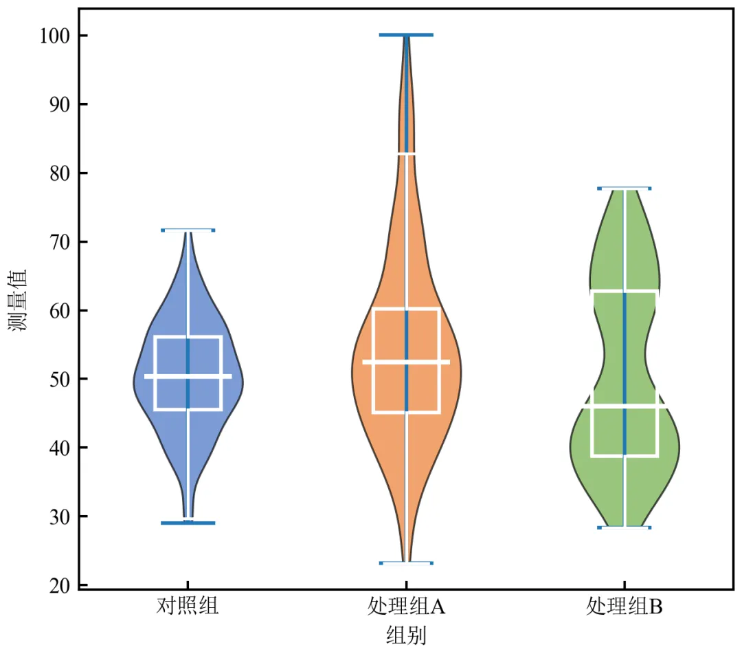
手动绘制箱线图元素可完全控制线条颜色、粗细,实现白色内嵌箱线图,与深色小提琴形成对比。
小提琴颜色半透明,内部结构清晰可见。
此方法适合需要高度定制化的出版级图表。
进阶2:小提琴图 + 散点叠加(展示所有数据点)
在小提琴图旁或内部叠加原始数据点,增强数据透明度,尤其适合样本量不大的情况。
import pandas as pdimport numpy as npimport matplotlib.pyplot as pltimport seaborn as snsdefset_academic_style(): plt.rcParams['font.family'] = ['Times New Roman', 'SimSun'] plt.rcParams['font.size'] = 9 plt.rcParams['axes.unicode_minus'] = False plt.rcParams['axes.linewidth'] = 1.0 plt.rcParams['xtick.major.width'] = 1.0 plt.rcParams['ytick.major.width'] = 1.0 plt.rcParams['xtick.major.size'] = 3.5 plt.rcParams['ytick.major.size'] = 3.5 plt.rcParams['xtick.direction'] = 'in' plt.rcParams['ytick.direction'] = 'in' plt.rcParams['legend.frameon'] = False plt.rcParams['pdf.fonttype'] = 42 plt.rcParams['savefig.dpi'] = 300set_academic_style()df = pd.read_csv('三组实验数据.csv')fig, ax = plt.subplots(figsize=(5.0, 4.0))# 绘制小提琴图(半透明)sns.violinplot(data=df, x='组别', y='测量值', inner=None, palette=['#4472C4', '#ED7D31', '#70AD47'], alpha=0.5, linewidth=0.8, ax=ax)# 叠加散点(带抖动)sns.stripplot(data=df, x='组别', y='测量值', jitter=0.15, size=3, alpha=0.6, palette=['#4472C4', '#ED7D31', '#70AD47'], ax=ax)ax.set_xlabel('组别')ax.set_ylabel('测量值')sns.despine()plt.tight_layout()plt.show()fig.savefig('小提琴图_散点叠加.pdf', bbox_inches='tight', pad_inches=0.05)fig.savefig('小提琴图_散点叠加.png', bbox_inches='tight', pad_inches=0.05)执行结果分析:
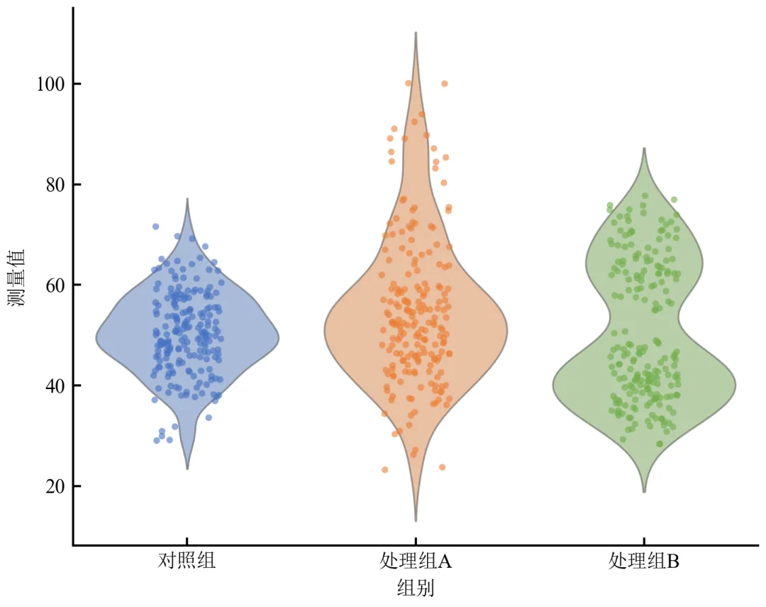
散点展示了每个样本的具体值,处理组B的双峰结构在散点图中表现为两个簇。
抖动(jitter)避免点重叠,但需注意不要误导分布形状;小提琴轮廓提供准确密度估计。
适合小样本(n<200)或需要展示所有数据点的场景。
进阶3:分组小提琴图(按第二类别细分)
当存在两个分类变量时,使用hue参数绘制分组小提琴图。
import pandas as pdimport numpy as npimport matplotlib.pyplot as pltimport seaborn as snsdefset_academic_style(): plt.rcParams['font.family'] = ['Times New Roman', 'SimSun'] plt.rcParams['font.size'] = 9 plt.rcParams['axes.unicode_minus'] = False plt.rcParams['axes.linewidth'] = 1.0 plt.rcParams['xtick.major.width'] = 1.0 plt.rcParams['ytick.major.width'] = 1.0 plt.rcParams['xtick.major.size'] = 3.5 plt.rcParams['ytick.major.size'] = 3.5 plt.rcParams['xtick.direction'] = 'in' plt.rcParams['ytick.direction'] = 'in' plt.rcParams['legend.frameon'] = False plt.rcParams['pdf.fonttype'] = 42 plt.rcParams['savefig.dpi'] = 300set_academic_style()# 扩展数据:添加“时间点”变量np.random.seed(2024)df = pd.read_csv('三组实验数据.csv')# 复制数据,增加时间点维度df_time = df.copy()df_time['时间点'] = 'T0'df2 = df.copy()df2['时间点'] = 'T1'df2['测量值'] = df2['测量值'] * np.random.uniform(1.1, 1.3, len(df2)) # T1整体上移df_long = pd.concat([df_time, df2], ignore_index=True)fig, ax = plt.subplots(figsize=(6.0, 4.0))sns.violinplot(data=df_long, x='组别', y='测量值', hue='时间点', split=False, inner='box', palette='Set2', linewidth=0.8, ax=ax)ax.set_xlabel('组别')ax.set_ylabel('测量值')ax.legend(title='时间点', frameon=False, fontsize=8)sns.despine()plt.tight_layout()plt.show()fig.savefig('小提琴图_分组对比.pdf', bbox_inches='tight', pad_inches=0.05)fig.savefig('小提琴图_分组对比.png', bbox_inches='tight', pad_inches=0.05)执行结果分析:
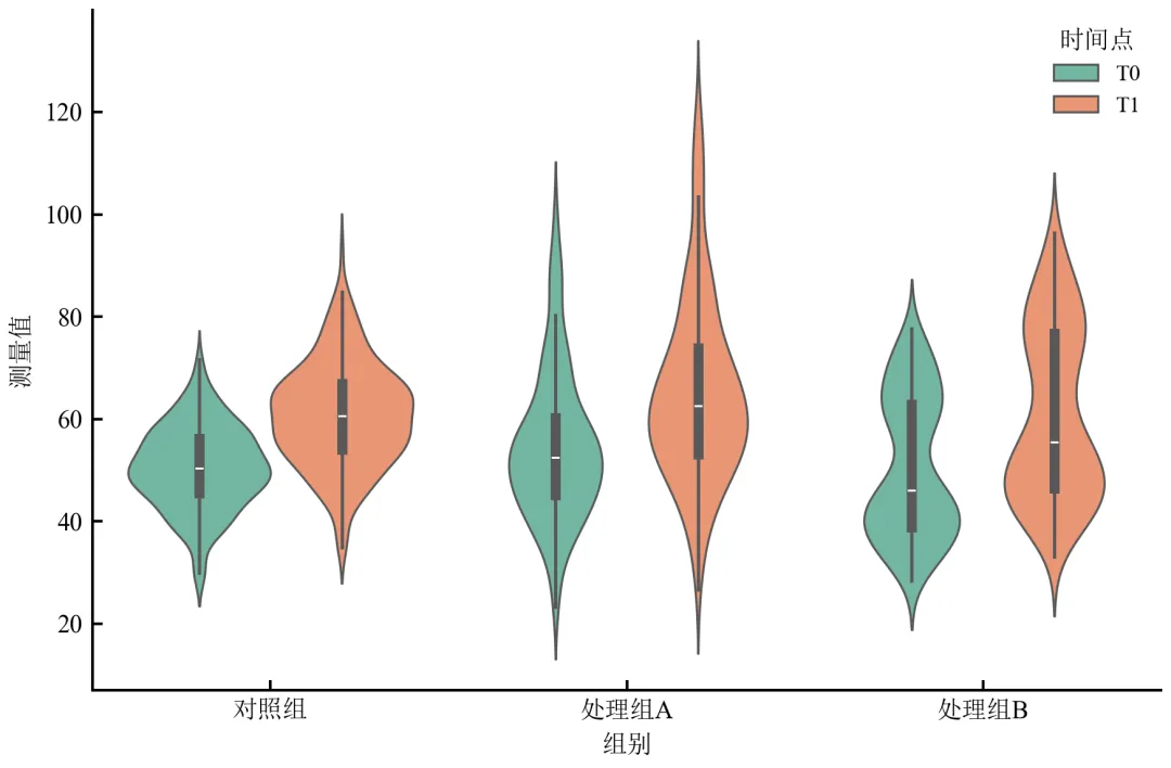
每组内并排展示T0和T1的小提琴图,直观比较时间效应。
可通过split=True将两个时间点的小提琴在组内左右对称绘制(需两组hue),适合配对比较。
适用于多因素实验设计的数据展示。
进阶4:调整核密度带宽(bw参数)优化小提琴平滑度
小提琴图的平滑程度由核密度估计的带宽决定,通过调整带宽可突出或抑制分布细节。
import pandas as pdimport numpy as npimport matplotlib.pyplot as pltimport seaborn as snsdefset_academic_style(): plt.rcParams['font.family'] = ['Times New Roman', 'SimSun'] plt.rcParams['font.size'] = 9 plt.rcParams['axes.unicode_minus'] = False plt.rcParams['axes.linewidth'] = 1.0 plt.rcParams['xtick.major.width'] = 1.0 plt.rcParams['ytick.major.width'] = 1.0 plt.rcParams['xtick.major.size'] = 3.5 plt.rcParams['ytick.major.size'] = 3.5 plt.rcParams['xtick.direction'] = 'in' plt.rcParams['ytick.direction'] = 'in' plt.rcParams['legend.frameon'] = False plt.rcParams['pdf.fonttype'] = 42 plt.rcParams['savefig.dpi'] = 300set_academic_style()df = pd.read_csv('三组实验数据.csv')# 使用处理组B(双峰)演示带宽影响data_b = df[df['组别'] == '处理组B']['测量值'].valuesfig, axes = plt.subplots(1, 3, figsize=(8.0, 3.5))bw_values = [0.5, 2.0, 5.0] # 相对于标准带宽的缩放因子for ax, bw in zip(axes, bw_values):# 使用matplotlib的violinplot,可控制带宽 parts = ax.violinplot([data_b], positions=[1], bw_method=bw, showmeans=False, showmedians=False) parts['bodies'][0].set_facecolor('#70AD47') parts['bodies'][0].set_alpha(0.7)# 添加箱线信息 q1, med, q3 = np.percentile(data_b, [25, 50, 75]) ax.scatter(1, med, color='white', edgecolor='black', s=30, zorder=3) ax.plot([0.9, 1.1], [q1, q1], color='black', linewidth=1) ax.plot([0.9, 1.1], [q3, q3], color='black', linewidth=1) ax.plot([1, 1], [q1, q3], color='black', linewidth=1.5) ax.set_title(f'bw_method = {bw}') ax.set_xticks([1]) ax.set_xticklabels(['处理组B']) ax.set_ylabel('测量值') ax.set_xlim(0.5, 1.5)plt.tight_layout()plt.show()fig.savefig('小提琴图_带宽调整.pdf', bbox_inches='tight', pad_inches=0.05)fig.savefig('小提琴图_带宽调整.png', bbox_inches='tight', pad_inches=0.05)执行结果分析:
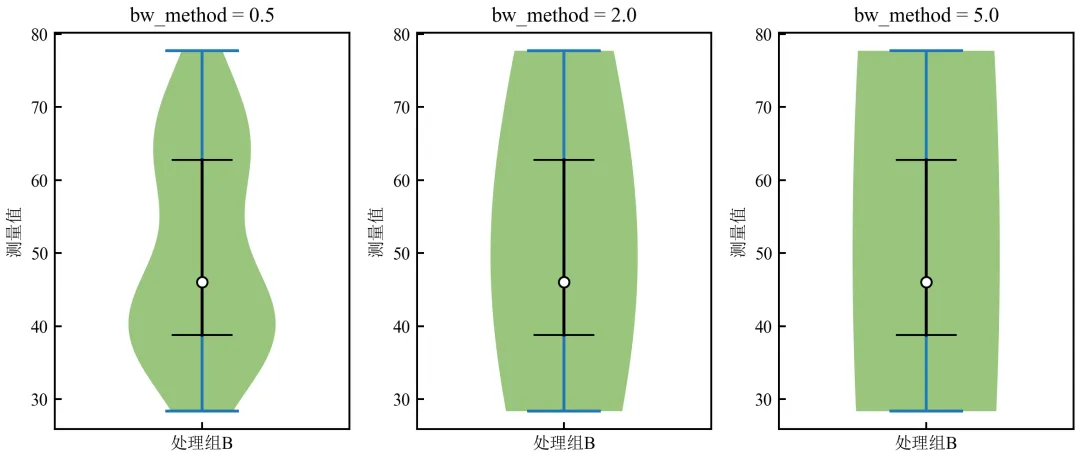
bw_method=0.5:带宽小,小提琴显示更多细节,双峰结构突出。
bw_method=2.0:适中带宽,双峰仍可见但更平滑。
bw_method=5.0:带宽过大,双峰被过度平滑,呈现单峰假象。
推荐使用Seaborn默认带宽或根据Scott规则自动选择,特殊情况下可手动调整以强调或抑制细节。
- END -随机文章
-
 10个月宝宝每天需要喝多少奶粉?
- 程序员的浪漫!用 Python 写一个满屏爱心弹窗,给 TA 一个超甜惊喜
- uv -- Python版本、环境、软件包管理工具
- 抽絲剝繭——python中bs4的幾個用法
- Python到底有多强?看完这些神级应用,我彻底跪了!(2026最新版)
- NotebookLM Python接口库上线 全面操控音频/视频/思维导图生成 突破网页端限制 支持Agent自动化流水线
- 用Python画一棵浪漫樱花树,递归+随机效果
- EC 数据驱动的颠簸指数计算全解析(Python 实现)
- Python ctypes:开启与硬件及操作系统 API 交互的钥匙
- Python 调用Kafka实例分析与应用
- Kali与编程: Kali Linux 无线安全测试工具命令速查手册
