机器学习--基础入门--08Python机器学习常见库
- 2026-07-01 23:11:16
Python机器学习常见库:掌握数据科学的四大神器
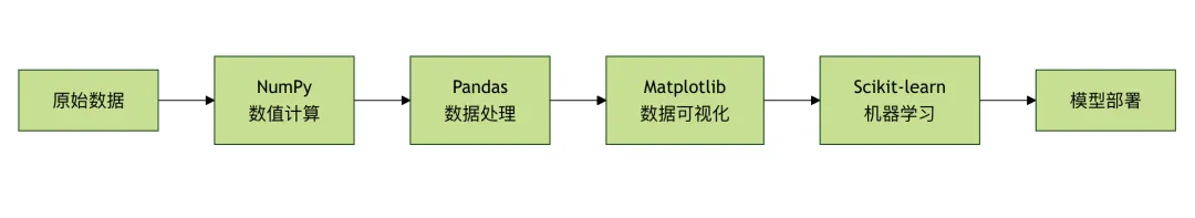
你已经配置好了环境,写下了第一行机器学习代码。现在,是时候认识你的"武器库"了——NumPy、Pandas、Matplotlib、Scikit-learn。这四个库构成了Python机器学习的核心生态,几乎所有的数据科学项目都绕不开它们。
但它们不是独立的工具,而是一个有机整体:NumPy提供数值计算基础,Pandas处理结构化数据,Matplotlib绘制可视化图表,Scikit-learn实现机器学习建模。数据在这些库之间流转,形成完整的分析链路。本章将带你深入理解每个库的核心功能与设计哲学,并通过实战项目融会贯通。准备好了吗?让我们打开这个"工具箱"!
开篇:机器学习开发者的工具箱
库之间的依赖关系
1 2 3 4 5 6 7 8 9 10 11 12 13 14 15 16 17 18 ┌─────────────────────────────────────────────────────┐│ 你的机器学习项目 │└─────────────────────────────────────────────────────┘ ↓┌─────────────────────────────────────────────────────┐│ Scikit-learn (建模与预测) ││ 内部使用 NumPy 数组,接受 Pandas DataFrame 输入 │└─────────────────────────────────────────────────────┘ ↓ ↓┌─────────────────────┐ ┌─────────────────────────┐│ Pandas (数据处理) │ │ Matplotlib (可视化) ││ 底层基于 NumPy 数组 │ │ 可直接绘制 DataFrame │└─────────────────────┘ └─────────────────────────┘ ↓ ↓┌─────────────────────────────────────────────────────┐│ NumPy (高性能数值计算基础层) ││ 用 C 实现的底层,提供 Python 接口 │└─────────────────────────────────────────────────────┘
这四个库是一个有机整体,不是相互独立的工具。数据通常在这四个库之间循环往复:
• NumPy 数组 → Pandas DataFrame(加标签、加索引) • Pandas DataFrame → Matplotlib(可视化) • Pandas DataFrame → Scikit-learn(建模,自动转为 NumPy 数组)
原生 Python vs 科学计算库:性能对比
1 2 3 4 5 6 7 8 9 10 11 12 13 14 15 # 场景:计算 100 万个数的平方和# ❌ 方法1:使用 Python 原生列表和循环import time# 创建包含 100 万个数的列表python_list = list(range(1_000_000))start = time.time()result = 0for num in python_list: result += num ** 2end = time.time()print(f"Python 循环耗时: {end - start:.4f} 秒")# Python 循环耗时: 0.2355 秒
1 2 3 4 5 6 7 8 9 10 11 12 # ✅ 方法2:使用 NumPy 向量化运算import numpy as npimport time# 创建 NumPy 数组numpy_array = np.arange(1_000_000)start = time.time()result = np.sum(numpy_array ** 2)end = time.time()print(f"NumPy 向量化耗时: {end - start:.4f} 秒")# NumPy 向量化耗时: 0.0053 秒
为什么 NumPy 这么快?
| 内存布局 | ||
| 类型检查 | ||
| 循环开销 | ||
| 缓存友好 |
第一章:NumPy
1.1 定义
NumPy(Numerical Python)的设计围绕三个核心原则:
1. 同质性(Homogeneity):数组中所有元素必须是相同类型 2. 向量化:用整体运算替代逐元素循环 3. 内存效率:紧凑存储,避免 Python 对象的开销
数据结构:ndarray(N-dimensional array)
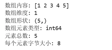
ndarray 是 NumPy 的核心,也是掌握 NumPy 的关键:
1 2 3 4 5 6 7 8 9 10 import numpy as np# 创建一个简单的一维数组arr = np.array([1, 2, 3, 4, 5])print(f"数组内容: {arr}")print(f"数组维度: {arr.ndim}") # 预期输出: 1print(f"数组形状: {arr.shape}") # 预期输出: (5,)print(f"数组元素类型: {arr.dtype}") # 预期输出: int64print(f"元素总数: {arr.size}") # 预期输出: 5print(f"每个元素字节大小: {arr.itemsize}") # 预期输出: 8
ndarray 的关键属性速查:
ndim | ||
shape | ||
dtype | ||
size | ||
itemsize | ||
nbytes |
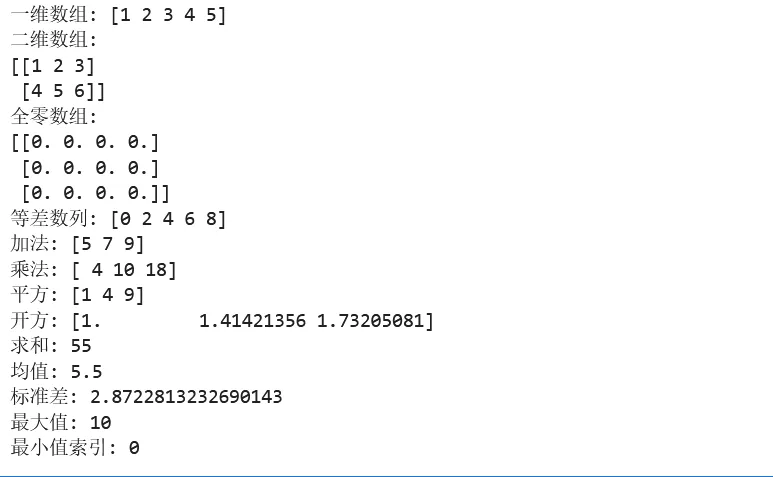
1.2 入门小测一份
1 2 3 4 5 6 7 8 9 10 11 12 13 14 15 16 17 18 19 20 21 22 23 24 25 26 27 28 29 30 31 32 33 34 35 36 37 import numpy as np# ===== 第一步:创建数组 =====# 从列表创建data = [1, 2, 3, 4, 5]arr = np.array(data)print(f"一维数组: {arr}")# 创建二维数组(矩阵)matrix = np.array([[1, 2, 3], [4, 5, 6]])print(f"二维数组:\n{matrix}")# ===== 第二步:快速创建特殊数组 =====zeros = np.zeros((3, 4)) # 3行4列的全0数组ones = np.ones((2, 3)) # 2行3列的全1数组range_arr = np.arange(0, 10, 2) # 等差数列: [0, 2, 4, 6, 8]linspace_arr = np.linspace(0, 1, 5) # 0到1之间等分5个点print(f"全零数组:\n{zeros}")print(f"等差数列: {range_arr}")# ===== 第三步:数组运算 =====a = np.array([1, 2, 3])b = np.array([4, 5, 6])print(f"加法: {a + b}") # [5, 7, 9]print(f"乘法: {a * b}") # [4, 10, 18]print(f"平方: {a ** 2}") # [1, 4, 9]print(f"开方: {np.sqrt(a)}") # [1., 1.41, 1.73]# ===== 第四步:统计运算 =====data = np.array([1, 2, 3, 4, 5, 6, 7, 8, 9, 10])print(f"求和: {data.sum()}") # 55print(f"均值: {data.mean()}") # 5.5print(f"标准差: {data.std()}") # 2.87print(f"最大值: {data.max()}") # 10print(f"最小值索引: {data.argmin()}") # 0
1.3 实例:典型应用场景
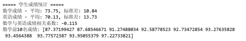
示例 1:数据生成与随机采样
1 2 3 4 5 6 7 8 9 10 11 12 13 14 15 16 17 18 19 20 21 22 23 24 25 26 27 import numpy as npnp.random.seed(42) # 设置随机种子,确保结果可复现# ===== 场景:模拟学生考试成绩数据 =====n_students = 100# 生成正态分布的成绩数据# 假设平均分 75,标准差 12math_scores = np.random.normal(75, 12, n_students)english_scores = np.random.normal(70, 15, n_students)# 确保分数在 0-100 之间math_scores = np.clip(math_scores, 0, 100)english_scores = np.clip(english_scores, 0, 100)print("===== 学生成绩统计 =====")print(f"数学成绩 - 平均: {math_scores.mean():.2f}, 标准差: {math_scores.std():.2f}")print(f"英语成绩 - 平均: {english_scores.mean():.2f}, 标准差: {english_scores.std():.2f}")# 计算两科成绩的相关系数correlation = np.corrcoef(math_scores, english_scores)[0, 1]print(f"数学与英语成绩相关系数: {correlation:.3f}")# 预期输出: 相关系数约 0.0~0.3(因为是独立生成的随机数据)# 找出数学成绩前 10 名的索引top_10_indices = np.argsort(math_scores)[-10:]print(f"数学前10名成绩: {math_scores[top_10_indices]}")
示例 2:图像数据处理基础
1 2 3 4 5 6 7 8 9 10 11 12 13 14 15 16 17 18 19 20 21 22 23 24 25 import numpy as np# ===== 场景:理解图像就是数组 =====# 创建一个 100x100 的灰度图像(单通道)height, width = 100, 100image = np.zeros((height, width), dtype=np.uint8)# 在中心画一个白色圆center_y, center_y = height // 2, width // 2radius = 30# 生成坐标网格(进阶:广播机制)y, x = np.ogrid[:height, :width]mask = (x - center_y)**2 + (y - center_y)**2 <= radius**2# 应用掩码image[mask] = 255print(f"图像形状: {image.shape}")print(f"图像数据类型: {image.dtype}")print(f"白色像素数量: {np.sum(image == 255)}")# 简单的图像处理:翻转image_flipped = image[::-1, :] # 垂直翻转image_mirrored = image[:, ::-1] # 水平镜像

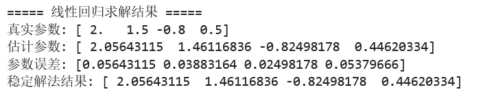
示例 3:数值计算与线性代数
1 2 3 4 5 6 7 8 9 10 11 12 13 14 15 16 17 18 19 20 21 22 23 24 25 26 27 28 29 30 31 32 33 import numpy as np# ===== 场景:线性回归的矩阵解法 =====# 线性回归的解析解: θ = (X^T X)^(-1) X^T y# 生成模拟数据np.random.seed(42)n_samples = 100n_features = 3# 特征矩阵(添加偏置列)X = np.random.randn(n_samples, n_features)X_with_bias = np.c_[np.ones(n_samples), X] # 添加全1列作为偏置# 真实参数true_theta = np.array([2.0, 1.5, -0.8, 0.5])# 生成目标变量(添加噪声)y = X_with_bias @ true_theta + np.random.randn(n_samples) * 0.5# 使用正规方程求解# θ = (X^T X)^(-1) X^T ytheta_hat = np.linalg.inv(X_with_bias.T @ X_with_bias) @ X_with_bias.T @ yprint("===== 线性回归求解结果 =====")print(f"真实参数: {true_theta}")print(f"估计参数: {theta_hat}")print(f"参数误差: {np.abs(true_theta - theta_hat)}")# 预期输出: 估计参数应接近真实参数# 更稳定的解法(推荐)theta_hat_stable = np.linalg.lstsq(X_with_bias, y, rcond=None)[0]print(f"稳定解法结果: {theta_hat_stable}")
1.4 广播机制与内存布局
广播机制
💡 广播:让不同形状的数组进行运算的规则,无需显式复制数据。
广播规则:
1. 从右向左比较各维度 2. 维度相等,或其中一个为 1,则兼容 3. 缺失的维度视为 1
1 2 3 4 5 6 7 8 9 10 11 12 13 14 15 16 17 18 19 20 21 22 23 24 25 import numpy as np# 示例1:数组与标量a = np.array([1, 2, 3])b = 10print(f"数组 + 标量: {a + b}") # [11, 12, 13]# 示例2:不同形状的数组A = np.array([[1, 2, 3], # shape: (2, 3) [4, 5, 6]])B = np.array([10, 20, 30]) # shape: (3,)# B 自动扩展为 [[10, 20, 30], [10, 20, 30]]print(f"矩阵 + 向量:\n{A + B}")# 示例3:列向量与行向量col = np.array([[1], [2], [3]]) # shape: (3, 1)row = np.array([10, 20]) # shape: (2,)# 结果是 (3, 2) 矩阵print(f"列向量 × 行向量:\n{col + row}")# 预期输出:# [[11, 21],# [12, 22],# [13, 23]]
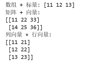
广播过程:
1 2 3 4 5 6 7 8 9 10 数组 A (3, 1): 数组 B (1, 4): 结果 (3, 4):[[1] [[10 20 30 40]] [[11 21 31 41] [2] + [12 22 32 42] [3]] [13 23 33 43]]扩展过程:A 变为: B 变为:[[1 1 1 1] [[10 20 30 40] [2 2 2 2] + [10 20 30 40] [3 3 3 3]] [10 20 30 40]]
1.5 NumPy 常用功能
数组创建
np.array() | np.array([1, 2, 3]) | |
np.zeros() | np.zeros((3, 4)) | |
np.ones() | np.ones((2, 3)) | |
np.empty() | np.empty((2, 2)) | |
np.arange() | np.arange(0, 10, 2) | |
np.linspace() | np.linspace(0, 1, 5) | |
np.eye() | np.eye(3) | |
np.random.rand() | np.random.rand(3, 3) | |
np.random.randn() | np.random.randn(3, 3) |
数组操作
reshape() | arr.reshape(2, 3) | |
ravel()flatten() | arr.ravel() | |
transpose().T | arr.T | |
concatenate() | np.concatenate([a, b]) | |
split() | np.split(arr, 3) | |
squeeze() | arr.squeeze() |
数学运算
np.add/subtract/multiply/divide | np.add(a, b) | |
np.power() | np.power(a, 2) | |
np.sqrt() | np.sqrt(a) | |
np.exp() | np.exp(a) | |
np.log() | np.log(a) | |
np.sin/cos/tan | np.sin(a) | |
np.dot()@ | a @ b |
统计函数
sum() | arr.sum(axis=0) | |
mean() | arr.mean() | |
std()var() | arr.std() | |
min()max() | arr.max() | |
argmin()argmax() | arr.argmax() | |
cumsum() | arr.cumsum() | |
percentile() | np.percentile(arr, 50) |
第二章:Pandas
2.1 定义
Pandas 的名字来源于 Panel Data(面板数据),由 Wes McKinney 于 2008 年开发。其设计哲学包括:
1. 标签化索引:每行每列都有名字,不依赖位置索引 2. 对齐机制:运算时自动对齐标签,避免错位 3. 缺失值处理:内置对缺失值的优雅处理 4. 表格化思维:让数据操作接近 SQL 或 Excel 的思维模式
数据结构对比
| Series | |||
| DataFrame | |||
| Index |
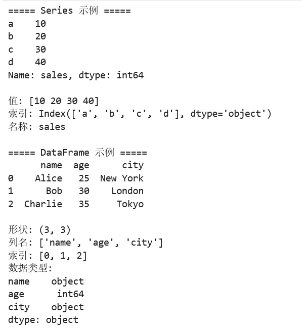
1 2 3 4 5 6 7 8 9 10 11 12 13 14 15 16 17 18 19 20 21 22 23 24 25 26 27 28 29 30 31 32 33 34 35 36 37 38 39 40 41 42 import pandas as pdimport numpy as np# ===== Series:带标签的一维数组 =====# 创建一个 Seriess = pd.Series([10, 20, 30, 40], index=['a', 'b', 'c', 'd'], name='sales')print("===== Series 示例 =====")print(s)# 预期输出:# a 10# b 20# c 30# d 40# Name: sales, dtype: int64print(f"\n值: {s.values}") # NumPy 数组print(f"索引: {s.index}") # Index 对象print(f"名称: {s.name}")# ===== DataFrame:表格型数据结构 =====# 创建 DataFramedf = pd.DataFrame({ 'name': ['Alice', 'Bob', 'Charlie'], 'age': [25, 30, 35], 'city': ['New York', 'London', 'Tokyo']})print("\n===== DataFrame 示例 =====")print(df)# 预期输出:# name age city# 0 Alice 25 New York# 1 Bob 30 London# 2 Charlie 35 Tokyoprint(f"\n形状: {df.shape}") # (3, 3)print(f"列名: {df.columns.tolist()}") # ['name', 'age', 'city']print(f"索引: {df.index.tolist()}") # [0, 1, 2]print(f"数据类型:\n{df.dtypes}")
DataFrame vs Python 字典列表对比:
1 2 3 4 5 6 7 8 9 10 11 12 13 14 15 16 17 18 19 20 21 22 23 24 25 26 27 # 场景:存储学生信息# ❌ 方法1:使用字典列表students_list = [ {'name': 'Alice', 'age': 25, 'score': 85}, {'name': 'Bob', 'age': 30, 'score': 90}, {'name': 'Charlie', 'age': 35, 'score': 78}]# 获取所有年龄 - 需要循环ages = [s['age'] for s in students_list]# 计算平均分 - 需要手动计算avg_score = sum(s['score'] for s in students_list) / len(students_list)# ✅ 方法2:使用 DataFrameimport pandas as pddf = pd.DataFrame(students_list)# 获取所有年龄 - 直接取列ages = df['age']# 计算平均分 - 内置方法avg_score = df['score'].mean()# 筛选高分学生 - 链式操作high_scorers = df[df['score'] > 80]
2.2 快速入门小测
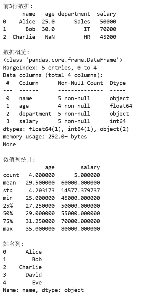
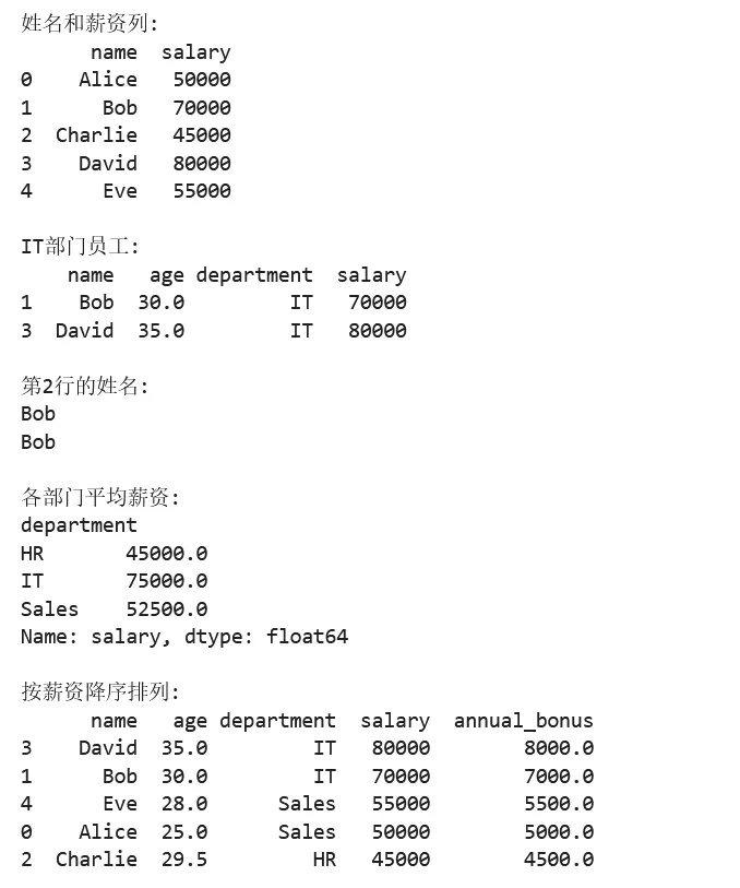
1 2 3 4 5 6 7 8 9 10 11 12 13 14 15 16 17 18 19 20 21 22 23 24 25 26 27 28 29 30 31 32 33 34 35 36 37 38 39 40 41 42 43 44 45 46 47 48 49 50 51 52 53 54 import pandas as pdimport numpy as np# ===== 第一步:创建 DataFrame =====# 从字典创建df = pd.DataFrame({ 'name': ['Alice', 'Bob', 'Charlie', 'David', 'Eve'], 'age': [25, 30, None, 35, 28], # 包含缺失值 'department': ['Sales', 'IT', 'HR', 'IT', 'Sales'], 'salary': [50000, 70000, 45000, 80000, 55000]})# ===== 第二步:查看数据 =====print("前3行数据:")print(df.head(3))print("\n数据概览:")print(df.info())print("\n数值列统计:")print(df.describe())# ===== 第三步:数据选择 =====# 选择单列print("\n姓名列:")print(df['name'])# 选择多列print("\n姓名和薪资列:")print(df[['name', 'salary']])# 按条件筛选print("\nIT部门员工:")print(df[df['department'] == 'IT'])# 使用 loc(标签索引)和 iloc(位置索引)print("\n第2行的姓名:")print(df.loc[1, 'name']) # 使用 locprint(df.iloc[1, 0]) # 使用 iloc# ===== 第四步:数据处理 =====# 填充缺失值df['age'] = df['age'].fillna(df['age'].mean())# 添加新列df['annual_bonus'] = df['salary'] * 0.1# 分组统计print("\n各部门平均薪资:")print(df.groupby('department')['salary'].mean())# 排序print("\n按薪资降序排列:")print(df.sort_values('salary', ascending=False))
2.3 实例:典型应用场景
示例 1:数据清洗与预处理
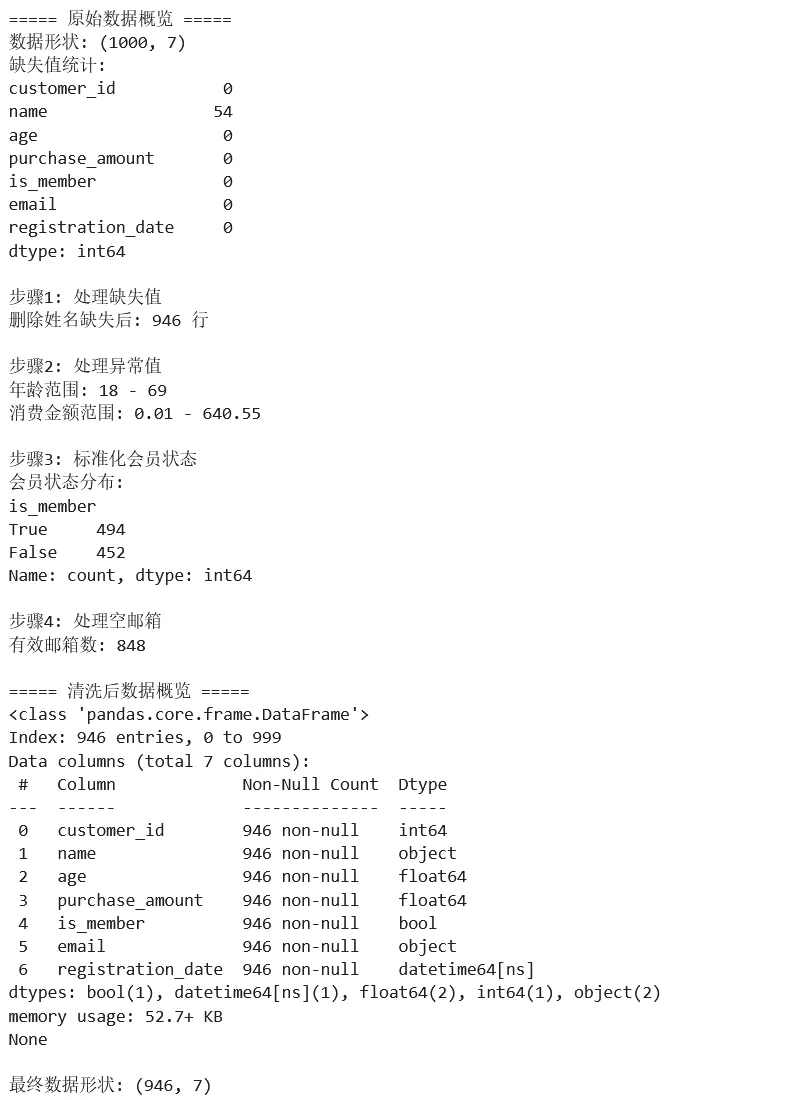
1 2 3 4 5 6 7 8 9 10 11 12 13 14 15 16 17 18 19 20 21 22 23 24 25 26 27 28 29 30 31 32 33 34 35 36 37 38 39 40 41 42 43 44 45 46 47 48 49 50 51 52 53 54 55 56 57 58 59 60 61 62 63 64 65 66 67 68 import pandas as pdimport numpy as np# ===== 场景:清洗脏数据 =====# 创建包含各种问题的模拟数据np.random.seed(42)n = 1000data = { 'customer_id': range(1, n + 1), 'name': [f'Customer_{i}' if np.random.random() > 0.05 else None for i in range(1, n + 1)], 'age': np.random.randint(18, 70, n), 'purchase_amount': np.random.exponential(100, n), 'is_member': np.random.choice([True, False, 'True', 'False', 'Yes', 'No'], n), 'email': [f'user{i}@example.com' if np.random.random() > 0.1 else '' for i in range(n)], 'registration_date': pd.date_range('2020-01-01', periods=n, freq='D').to_list()}df = pd.DataFrame(data)# 人为添加一些异常值df.loc[10:15, 'age'] = -1 # 不合法的年龄df.loc[20:25, 'purchase_amount'] = -100 # 负的消费金额print("===== 原始数据概览 =====")print(f"数据形状: {df.shape}")print(f"缺失值统计:\n{df.isnull().sum()}")# ===== 数据清洗步骤 =====# 1. 处理缺失值print("\n步骤1: 处理缺失值")# 删除姓名缺失的行(关键信息)df_clean = df.dropna(subset=['name'])print(f"删除姓名缺失后: {df_clean.shape[0]} 行")# 2. 处理异常值print("\n步骤2: 处理异常值")# 年龄异常:设为 NaN 然后用中位数填充df_clean = df_clean.copy()df_clean.loc[df_clean['age'] < 0, 'age'] = np.nandf_clean['age'] = df_clean['age'].fillna(df_clean['age'].median())# 消费金额异常:取绝对值df_clean['purchase_amount'] = df_clean['purchase_amount'].abs()print(f"年龄范围: {df_clean['age'].min():.0f} - {df_clean['age'].max():.0f}")print(f"消费金额范围: {df_clean['purchase_amount'].min():.2f} - {df_clean['purchase_amount'].max():.2f}")# 3. 标准化布尔值print("\n步骤3: 标准化会员状态")bool_mapping = {True: True, 'True': True, 'Yes': True, False: False, 'False': False, 'No': False}df_clean['is_member'] = df_clean['is_member'].map(bool_mapping)print(f"会员状态分布:\n{df_clean['is_member'].value_counts()}")# 4. 处理空邮箱print("\n步骤4: 处理空邮箱")df_clean.loc[df_clean['email'] == '', 'email'] = 'unknown@example.com'print(f"有效邮箱数: {(df_clean['email'] != 'unknown@example.com').sum()}")# 5. 数据类型转换df_clean['registration_date'] = pd.to_datetime(df_clean['registration_date'])print("\n===== 清洗后数据概览 =====")print(df_clean.info())print(f"\n最终数据形状: {df_clean.shape}")
示例 2:分组聚合与数据透视
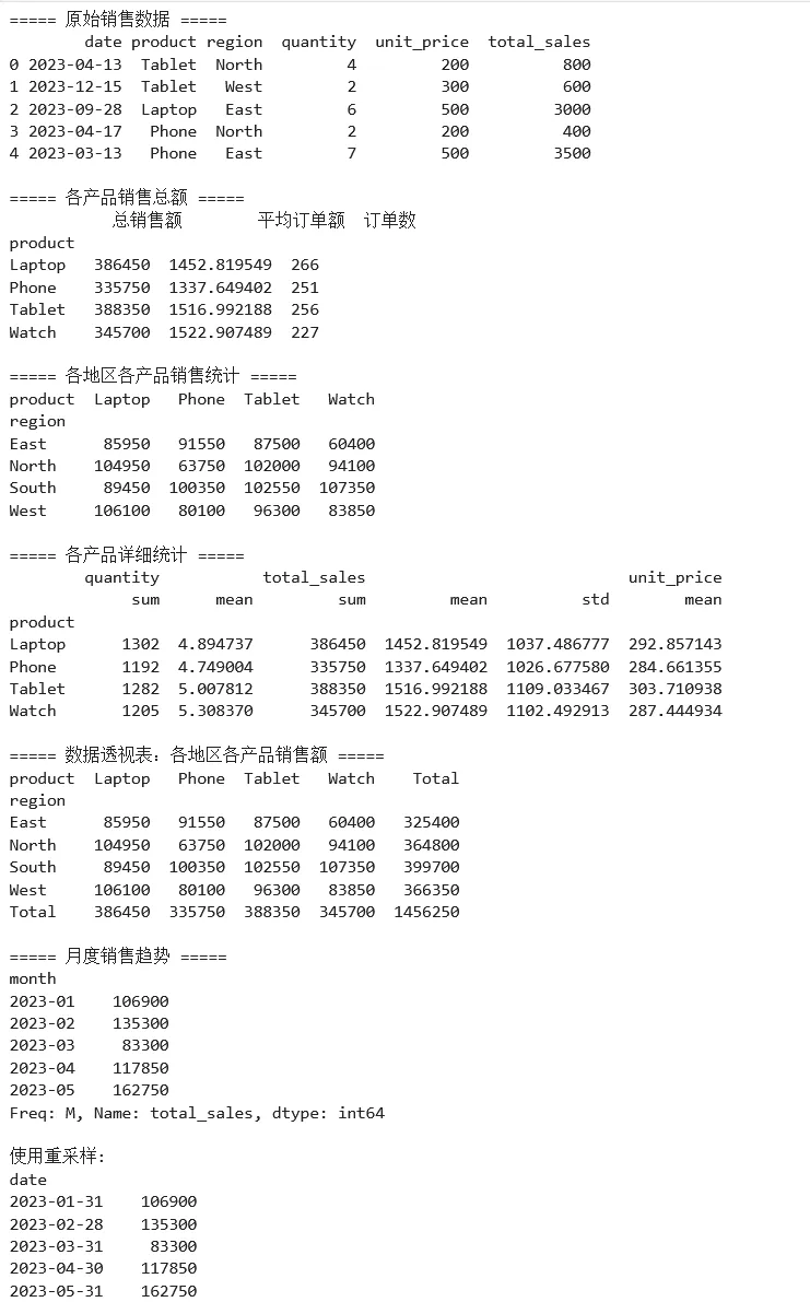
1 2 3 4 5 6 7 8 9 10 11 12 13 14 15 16 17 18 19 20 21 22 23 24 25 26 27 28 29 30 31 32 33 34 35 36 37 38 39 40 41 42 43 44 45 46 47 48 49 50 51 52 53 54 55 56 57 58 59 60 61 62 63 64 65 66 67 68 69 70 71 72 73 import pandas as pdimport numpy as np# ===== 场景:销售数据分析 =====# 创建模拟销售数据np.random.seed(42)dates = pd.date_range('2023-01-01', '2023-12-31', freq='D')products = ['Laptop', 'Phone', 'Tablet', 'Watch']regions = ['North', 'South', 'East', 'West']data = { 'date': np.random.choice(dates, 1000), 'product': np.random.choice(products, 1000), 'region': np.random.choice(regions, 1000), 'quantity': np.random.randint(1, 10, 1000), 'unit_price': np.random.choice([500, 300, 200, 150], 1000)}df = pd.DataFrame(data)df['total_sales'] = df['quantity'] * df['unit_price']print("===== 原始销售数据 =====")print(df.head())# ===== 分组聚合分析 =====# 1. 单列分组print("\n===== 各产品销售总额 =====")product_sales = df.groupby('product')['total_sales'].agg(['sum', 'mean', 'count'])product_sales.columns = ['总销售额', '平均订单额', '订单数']print(product_sales)# 2. 多列分组print("\n===== 各地区各产品销售统计 =====")region_product = df.groupby(['region', 'product'])['total_sales'].sum().unstack()print(region_product)# 3. 多种聚合函数print("\n===== 各产品详细统计 =====")product_stats = df.groupby('product').agg({ 'quantity': ['sum', 'mean'], 'total_sales': ['sum', 'mean', 'std'], 'unit_price': 'mean'})print(product_stats)# ===== 数据透视表 =====print("\n===== 数据透视表:各地区各产品销售额 =====")pivot_table = pd.pivot_table( df, values='total_sales', index='region', columns='product', aggfunc='sum', margins=True, # 添加合计 margins_name='Total')print(pivot_table)# ===== 时间序列分析 =====print("\n===== 月度销售趋势 =====")df['month'] = df['date'].dt.to_period('M')monthly_sales = df.groupby('month')['total_sales'].sum()print(monthly_sales.head())# 转换为 datetime 索引并重采样df_time = df.set_index('date')monthly_resample = df_time.resample('M')['total_sales'].sum()print("\n使用重采样:")print(monthly_resample.head())
示例 3:数据合并与连接
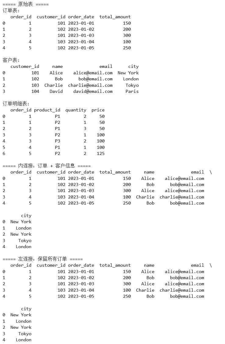
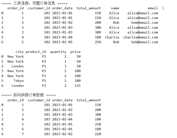
1 2 3 4 5 6 7 8 9 10 11 12 13 14 15 16 17 18 19 20 21 22 23 24 25 26 27 28 29 30 31 32 33 34 35 36 37 38 39 40 41 42 43 44 45 46 47 48 49 50 51 52 53 54 55 56 57 58 59 60 61 62 63 64 65 66 67 68 69 70 71 72 73 74 75 76 77 78 79 import pandas as pd# ===== 场景:电商订单数据分析 =====# 订单表orders = pd.DataFrame({ 'order_id': [1, 2, 3, 4, 5], 'customer_id': [101, 102, 101, 103, 102], 'order_date': pd.to_datetime(['2023-01-01', '2023-01-02', '2023-01-03', '2023-01-04', '2023-01-05']), 'total_amount': [150, 200, 300, 100, 250]})# 客户表customers = pd.DataFrame({ 'customer_id': [101, 102, 103, 104], 'name': ['Alice', 'Bob', 'Charlie', 'David'], 'email': ['alice@email.com', 'bob@email.com', 'charlie@email.com', 'david@email.com'], 'city': ['New York', 'London', 'Tokyo', 'Paris']})# 产品订单明细表order_items = pd.DataFrame({ 'order_id': [1, 1, 2, 3, 3, 4, 5], 'product_id': ['P1', 'P2', 'P1', 'P2', 'P3', 'P1', 'P2'], 'quantity': [2, 1, 3, 1, 2, 1, 2], 'price': [50, 50, 50, 100, 100, 100, 125]})print("===== 原始表 =====")print("订单表:")print(orders)print("\n客户表:")print(customers)print("\n订单明细表:")print(order_items)# ===== 合并操作 =====# 1. 内连接print("\n===== 内连接:订单 + 客户信息 =====")orders_with_customer = pd.merge( orders, customers, on='customer_id', how='inner')print(orders_with_customer)# 2. 左连接(保留所有订单,即使没有客户信息)print("\n===== 左连接:保留所有订单 =====")orders_all = pd.merge( orders, customers, on='customer_id', how='left')print(orders_all)# 3. 多表连接print("\n===== 三表连接:完整订单信息 =====")complete_orders = (orders .merge(customers, on='customer_id', how='left') .merge(order_items, on='order_id', how='left'))print(complete_orders)# 4. 拼接操作print("\n===== 纵向拼接订单数据 =====")orders_jan = orders[orders['order_date'].dt.month == 1]# 假设有2月数据orders_feb = pd.DataFrame({ 'order_id': [6, 7], 'customer_id': [101, 103], 'order_date': pd.to_datetime(['2023-02-01', '2023-02-02']), 'total_amount': [180, 220]})all_orders = pd.concat([orders_jan, orders_feb], ignore_index=True)print(all_orders)
2.4 Pandas 常用功能速查表
数据读取与写入
pd.read_csv() | sep, header, names, dtype, parse_dates | |
pd.read_excel() | sheet_name, header, usecols | |
pd.read_json() | orient, typ | |
pd.read_sql() | sql, con, index_col | |
df.to_csv() | index, encoding | |
df.to_excel() | sheet_name, index |
数据选择
df['col'] | df['name'] | |
df[['col1', 'col2']] | df[['name', 'age']] | |
df.loc[row, col] | df.loc[0:5, 'name'] | |
df.iloc[row, col] | df.iloc[0:5, 0] | |
df.at[row, col] | df.at[0, 'name'] | |
df.iat[row, col] | df.iat[0, 0] | |
df.query() | df.query('age > 30') |
数据清洗
df.dropna() | df.dropna(subset=['col']) | |
df.fillna() | df.fillna(0) | |
df.drop_duplicates() | df.drop_duplicates() | |
df.replace() | df.replace('old', 'new') | |
df.rename() | df.rename(columns={'old': 'new'}) | |
df.astype() | df['col'].astype(int) |
分组与聚合
df.groupby() | df.groupby('col') | |
agg() | df.groupby('col').agg({'num': 'sum'}) | |
transform() | df.groupby('col').transform('mean') | |
apply() | df.groupby('col').apply(func) | |
pivot_table() | pd.pivot_table(df, values='v', index='i', columns='c') |
第三章:Matplotlib
3.1 定义
Matplotlib 由 John D. Hunter 于 2003 年创建,设计灵感来自 MATLAB。其核心设计原则:
1. 渐进式复杂度:简单的事情简单做,复杂的事情能做 2. 面向对象:所有图形元素都是对象,可精细控制 3. 出版级质量:支持多种输出格式,满足学术出版需求
对象模型
理解 Matplotlib 的关键是理解其对象层级结构:
1 2 3 4 5 6 7 8 9 Figure (整个图形窗口)├── Axes (单个子图/绑图区域) ← 最核心的对象│ ├── XAxis, YAxis (坐标轴)│ │ ├── Tick (刻度)│ │ └── Label (轴标签)│ ├── Legend (图例)│ ├── Title (标题)│ └── 各种绘图元素 (Line2D, Patch, Text, Image, etc.)└── 其他子图...
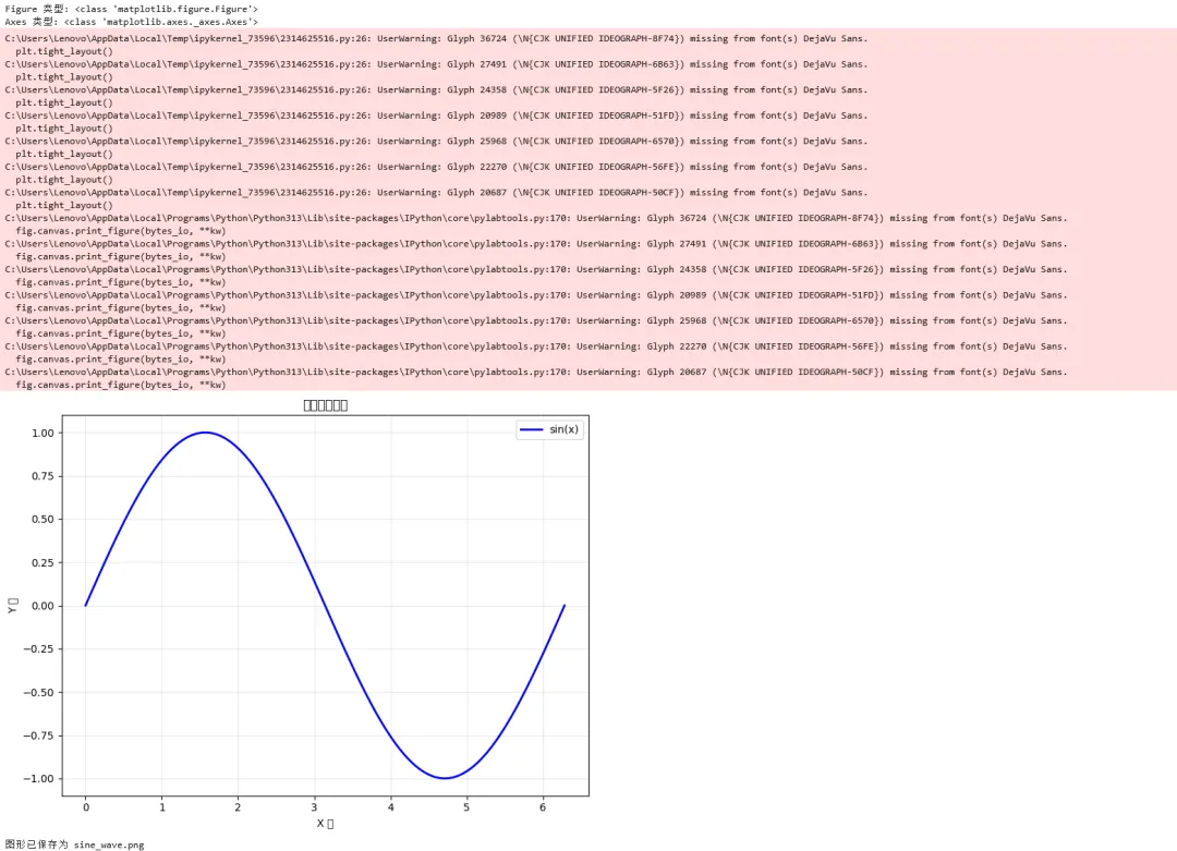
1 2 3 4 5 6 7 8 9 10 11 12 13 14 15 16 17 18 19 20 21 22 23 24 25 26 27 28 29 30 31 import matplotlib.pyplot as pltimport numpy as np# ===== 理解 Figure 和 Axes =====# 创建 Figure 和 Axesfig, ax = plt.subplots(figsize=(8, 6))# 查看对象类型print(f"Figure 类型: {type(fig)}")print(f"Axes 类型: {type(ax)}")# 创建示例数据x = np.linspace(0, 2*np.pi, 100)y = np.sin(x)# 在 Axes 上绘图ax.plot(x, y, label='sin(x)', color='blue', linewidth=2)ax.set_xlabel('X 轴')ax.set_ylabel('Y 轴')ax.set_title('正弦函数图像')ax.legend()ax.grid(True, alpha=0.3)# 显示图形plt.tight_layout()plt.show()# 保存图形fig.savefig('sine_wave.png', dpi=150, bbox_inches='tight')print("图形已保存为 sine_wave.png")
3.2 快速入门小测验
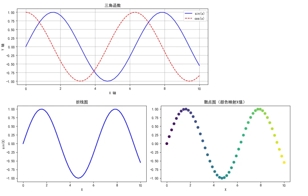
1 2 3 4 5 6 7 8 9 10 11 12 13 14 15 16 17 18 19 20 21 22 23 24 25 26 27 28 29 30 31 32 33 34 35 36 37 import matplotlib.pyplot as pltimport numpy as np# 设置中文显示(重要!)plt.rcParams['font.sans-serif'] = ['SimHei', 'Arial Unicode MS']plt.rcParams['axes.unicode_minus'] = False# ===== 方式1:快速绘图( pyplot 接口)=====x = np.linspace(0, 10, 50)y = np.sin(x)plt.figure(figsize=(10, 4))plt.plot(x, y, 'b-', label='sin(x)')plt.plot(x, np.cos(x), 'r--', label='cos(x)')plt.xlabel('X 轴')plt.ylabel('Y 轴')plt.title('三角函数')plt.legend()plt.grid(True)plt.show()# ===== 方式2:面向对象接口(推荐)=====fig, axes = plt.subplots(1, 2, figsize=(12, 4))# 子图1:折线图axes[0].plot(x, y, 'b-', linewidth=2)axes[0].set_title('折线图')axes[0].set_xlabel('X')axes[0].set_ylabel('sin(X)')# 子图2:散点图axes[1].scatter(x, y, c=x, cmap='viridis', s=50)axes[1].set_title('散点图(颜色映射X值)')axes[1].set_xlabel('X')plt.tight_layout()plt.show()
3.3 实例:常见图表类型
示例 1:探索性数据分析图表
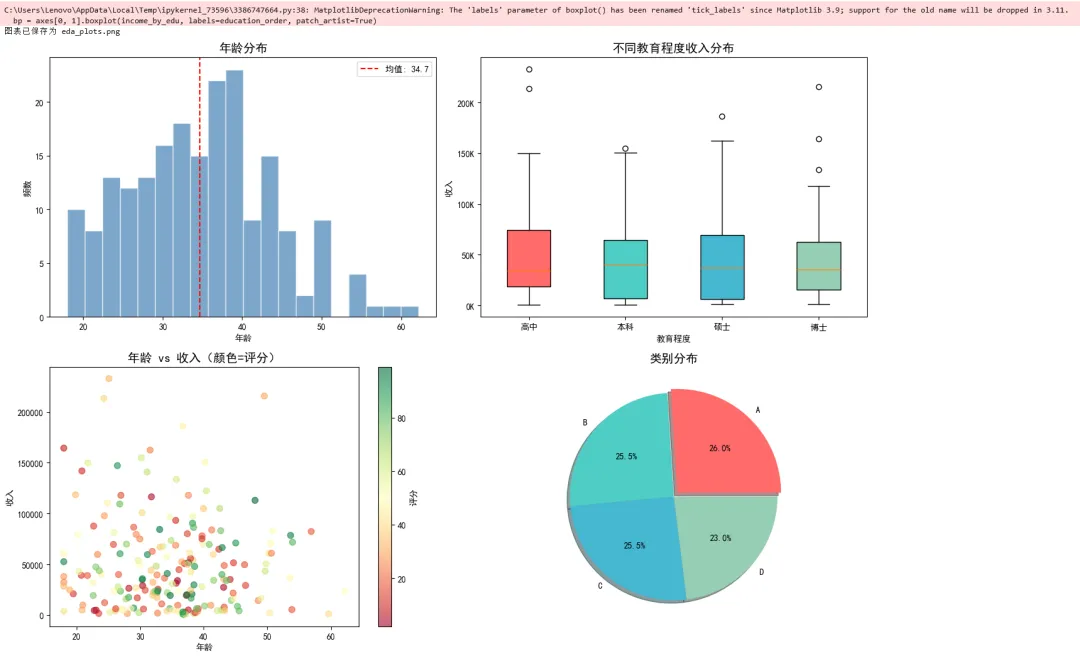
1 2 3 4 5 6 7 8 9 10 11 12 13 14 15 16 17 18 19 20 21 22 23 24 25 26 27 28 29 30 31 32 33 34 35 36 37 38 39 40 41 42 43 44 45 46 47 48 49 50 51 52 53 54 55 56 57 58 59 60 61 62 63 64 65 66 67 import matplotlib.pyplot as pltimport numpy as npimport pandas as pd# 设置中文显示plt.rcParams['font.sans-serif'] = ['SimHei', 'Arial Unicode MS']plt.rcParams['axes.unicode_minus'] = False# ===== 场景:数据探索可视化 =====# 生成模拟数据np.random.seed(42)n = 200data = { 'age': np.random.normal(35, 10, n).clip(18, 65), 'income': np.random.exponential(50000, n), 'education': np.random.choice(['高中', '本科', '硕士', '博士'], n), 'score': np.random.uniform(0, 100, n), 'category': np.random.choice(['A', 'B', 'C', 'D'], n)}df = pd.DataFrame(data)# 创建多子图进行探索fig, axes = plt.subplots(2, 2, figsize=(14, 10))# 子图1:直方图 - 年龄分布axes[0, 0].hist(df['age'], bins=20, color='steelblue', edgecolor='white', alpha=0.7)axes[0, 0].set_title('年龄分布', fontsize=14)axes[0, 0].set_xlabel('年龄')axes[0, 0].set_ylabel('频数')axes[0, 0].axvline(df['age'].mean(), color='red', linestyle='--', label=f'均值: {df["age"].mean():.1f}')axes[0, 0].legend()# 子图2:箱线图 - 不同教育程度的收入education_order = ['高中', '本科', '硕士', '博士']income_by_edu = [df[df['education'] == edu]['income'] for edu in education_order]bp = axes[0, 1].boxplot(income_by_edu, labels=education_order, patch_artist=True)colors = ['#FF6B6B', '#4ECDC4', '#45B7D1', '#96CEB4']for patch, color in zip(bp['boxes'], colors): patch.set_facecolor(color)axes[0, 1].set_title('不同教育程度收入分布', fontsize=14)axes[0, 1].set_xlabel('教育程度')axes[0, 1].set_ylabel('收入')axes[0, 1].yaxis.set_major_formatter(plt.FuncFormatter(lambda x, p: f'{x/1000:.0f}K'))# 子图3:散点图 - 年龄与收入的关系scatter = axes[1, 0].scatter(df['age'], df['income'], c=df['score'], cmap='RdYlGn', alpha=0.6, s=50)axes[1, 0].set_title('年龄 vs 收入(颜色=评分)', fontsize=14)axes[1, 0].set_xlabel('年龄')axes[1, 0].set_ylabel('收入')cbar = plt.colorbar(scatter, ax=axes[1, 0])cbar.set_label('评分')# 子图4:饼图 - 类别分布category_counts = df['category'].value_counts()axes[1, 1].pie(category_counts, labels=category_counts.index, autopct='%1.1f%%', colors=['#FF6B6B', '#4ECDC4', '#45B7D1', '#96CEB4'], explode=[0.05, 0, 0, 0], shadow=True)axes[1, 1].set_title('类别分布', fontsize=14)plt.tight_layout()plt.savefig('eda_plots.png', dpi=150, bbox_inches='tight')print("图表已保存为 eda_plots.png")plt.show()
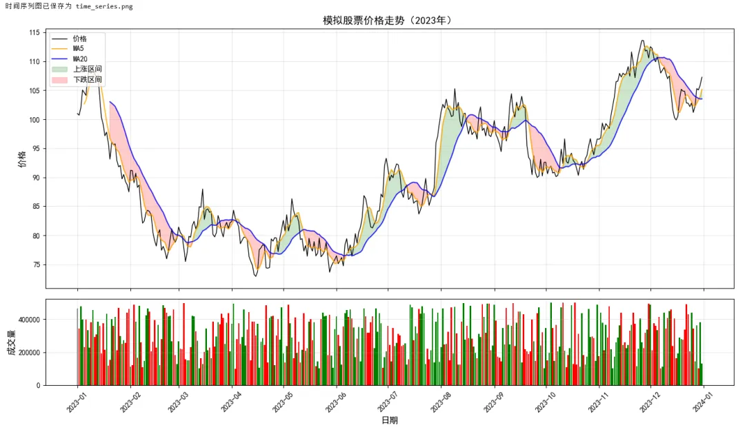
示例 2:时间序列可视化
1 2 3 4 5 6 7 8 9 10 11 12 13 14 15 16 17 18 19 20 21 22 23 24 25 26 27 28 29 30 31 32 33 34 35 36 37 38 39 40 41 42 43 44 45 46 47 48 49 50 51 52 53 54 55 56 57 58 59 60 61 62 63 64 65 66 67 import matplotlib.pyplot as pltimport pandas as pdimport numpy as np# ===== 场景:股票/销售时间序列 =====# 生成模拟时间序列数据np.random.seed(42)dates = pd.date_range('2023-01-01', '2023-12-31', freq='D')n = len(dates)# 模拟股票价格(随机游走)price = 100 + np.cumsum(np.random.randn(n) * 2)volume = np.random.randint(100000, 500000, n)# 创建 DataFramedf = pd.DataFrame({ 'date': dates, 'price': price, 'volume': volume, 'ma5': pd.Series(price).rolling(5).mean(), # 5日均线 'ma20': pd.Series(price).rolling(20).mean() # 20日均线})# ===== 绘制双轴图 =====fig, (ax1, ax2) = plt.subplots(2, 1, figsize=(14, 8), gridspec_kw={'height_ratios': [3, 1]}, sharex=True)# 上图:价格走势ax1.plot(df['date'], df['price'], label='价格', color='black', linewidth=1)ax1.plot(df['date'], df['ma5'], label='MA5', color='orange', linewidth=1.5, alpha=0.8)ax1.plot(df['date'], df['ma20'], label='MA20', color='blue', linewidth=1.5, alpha=0.8)# 填充区域ax1.fill_between(df['date'], df['ma5'], df['ma20'], where=(df['ma5'] > df['ma20']), color='green', alpha=0.2, label='上涨区间')ax1.fill_between(df['date'], df['ma5'], df['ma20'], where=(df['ma5'] < df['ma20']), color='red', alpha=0.2, label='下跌区间')ax1.set_ylabel('价格', fontsize=12)ax1.set_title('模拟股票价格走势(2023年)', fontsize=14)ax1.legend(loc='upper left')ax1.grid(True, alpha=0.3)# 下图:成交量柱状图colors = ['green' if df['price'].iloc[i] > df['price'].iloc[i-1] else 'red' for i in range(1, len(df))]colors = ['gray'] + colors # 第一天没有前一天,设为灰色ax2.bar(df['date'], df['volume'], color=colors, width=0.8)ax2.set_ylabel('成交量', fontsize=12)ax2.set_xlabel('日期', fontsize=12)ax2.grid(True, alpha=0.3)# 格式化 x 轴日期ax2.xaxis.set_major_locator(plt.matplotlib.dates.MonthLocator())ax2.xaxis.set_major_formatter(plt.matplotlib.dates.DateFormatter('%Y-%m'))plt.xticks(rotation=45)plt.tight_layout()plt.savefig('time_series.png', dpi=150, bbox_inches='tight')print("时间序列图已保存为 time_series.png")plt.show()
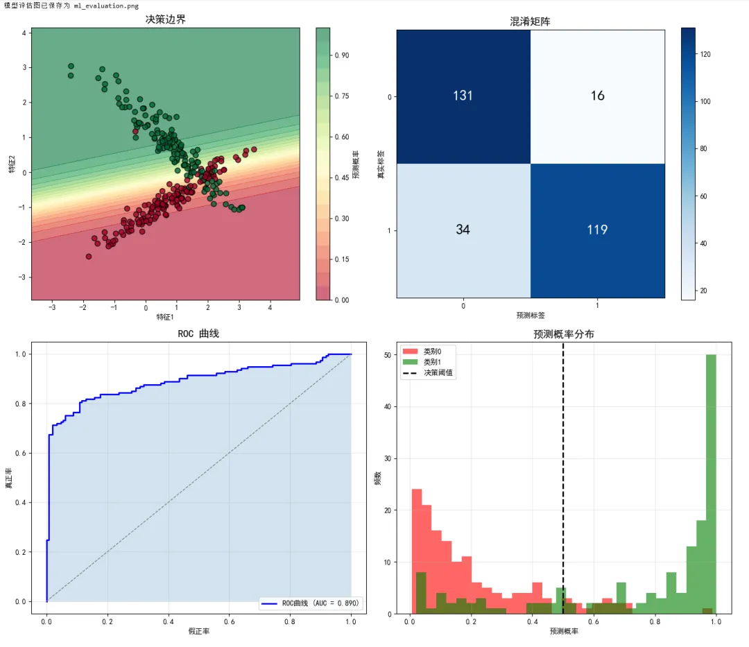
示例 3:机器学习结果可视化
1 2 3 4 5 6 7 8 9 10 11 12 13 14 15 16 17 18 19 20 21 22 23 24 25 26 27 28 29 30 31 32 33 34 35 36 37 38 39 40 41 42 43 44 45 46 47 48 49 50 51 52 53 54 55 56 57 58 59 60 61 62 63 64 65 66 67 68 69 70 71 72 73 74 75 76 77 78 79 80 81 82 83 84 85 86 87 88 89 import matplotlib.pyplot as pltimport numpy as npfrom sklearn.datasets import make_classificationfrom sklearn.model_selection import train_test_splitfrom sklearn.linear_model import LogisticRegressionfrom sklearn.metrics import confusion_matrix, roc_curve, auc# 设置中文显示plt.rcParams['font.sans-serif'] = ['SimHei', 'Arial Unicode MS']plt.rcParams['axes.unicode_minus'] = False# ===== 场景:分类模型评估可视化 =====# 生成分类数据X, y = make_classification(n_samples=1000, n_features=2, n_redundant=0, n_informative=2, n_clusters_per_class=1, class_sep=0.8, random_state=42)X_train, X_test, y_train, y_test = train_test_split(X, y, test_size=0.3, random_state=42)# 训练模型model = LogisticRegression()model.fit(X_train, y_train)# 预测y_pred = model.predict(X_test)y_prob = model.predict_proba(X_test)[:, 1]# ===== 创建评估图表 =====fig, axes = plt.subplots(2, 2, figsize=(14, 12))# 子图1:决策边界x_min, x_max = X[:, 0].min() - 1, X[:, 0].max() + 1y_min, y_max = X[:, 1].min() - 1, X[:, 1].max() + 1xx, yy = np.meshgrid(np.linspace(x_min, x_max, 100), np.linspace(y_min, y_max, 100))Z = model.predict_proba(np.c_[xx.ravel(), yy.ravel()])[:, 1]Z = Z.reshape(xx.shape)contour = axes[0, 0].contourf(xx, yy, Z, levels=20, cmap='RdYlGn', alpha=0.6)axes[0, 0].scatter(X_test[:, 0], X_test[:, 1], c=y_test, cmap='RdYlGn', edgecolors='black', s=50, alpha=0.8)axes[0, 0].set_title('决策边界', fontsize=14)axes[0, 0].set_xlabel('特征1')axes[0, 0].set_ylabel('特征2')plt.colorbar(contour, ax=axes[0, 0], label='预测概率')# 子图2:混淆矩阵cm = confusion_matrix(y_test, y_pred)im = axes[0, 1].imshow(cm, cmap='Blues')axes[0, 1].set_title('混淆矩阵', fontsize=14)axes[0, 1].set_xlabel('预测标签')axes[0, 1].set_ylabel('真实标签')axes[0, 1].set_xticks([0, 1])axes[0, 1].set_yticks([0, 1])# 添加数值标签for i in range(2): for j in range(2): axes[0, 1].text(j, i, cm[i, j], ha='center', va='center', fontsize=20, color='white' if cm[i, j] > cm.max()/2 else 'black')plt.colorbar(im, ax=axes[0, 1])# 子图3:ROC 曲线fpr, tpr, thresholds = roc_curve(y_test, y_prob)roc_auc = auc(fpr, tpr)axes[1, 0].plot(fpr, tpr, color='blue', linewidth=2, label=f'ROC曲线 (AUC = {roc_auc:.3f})')axes[1, 0].plot([0, 1], [0, 1], color='gray', linestyle='--', linewidth=1)axes[1, 0].fill_between(fpr, tpr, alpha=0.2)axes[1, 0].set_title('ROC 曲线', fontsize=14)axes[1, 0].set_xlabel('假正率')axes[1, 0].set_ylabel('真正率')axes[1, 0].legend(loc='lower right')axes[1, 0].grid(True, alpha=0.3)# 子图4:预测概率分布axes[1, 1].hist(y_prob[y_test == 0], bins=30, alpha=0.6, label='类别0', color='red')axes[1, 1].hist(y_prob[y_test == 1], bins=30, alpha=0.6, label='类别1', color='green')axes[1, 1].axvline(0.5, color='black', linestyle='--', linewidth=2, label='决策阈值')axes[1, 1].set_title('预测概率分布', fontsize=14)axes[1, 1].set_xlabel('预测概率')axes[1, 1].set_ylabel('频数')axes[1, 1].legend()axes[1, 1].grid(True, alpha=0.3)plt.tight_layout()plt.savefig('ml_evaluation.png', dpi=150, bbox_inches='tight')print("模型评估图已保存为 ml_evaluation.png")plt.show()
3.4 Matplotlib 常用功能速查表
基础绘图函数
plt.plot() | plt.plot(x, y, 'r--') | |
plt.scatter() | plt.scatter(x, y, c=colors) | |
plt.bar() | plt.bar(categories, values) | |
plt.hist() | plt.hist(data, bins=20) | |
plt.boxplot() | plt.boxplot(data) | |
plt.pie() | plt.pie(sizes, labels=labels) | |
plt.imshow() | plt.imshow(matrix, cmap='hot') | |
plt.contour() | plt.contour(X, Y, Z) |
图形元素设置
set_title() | ax.set_title('标题') | |
set_xlabel/ylabel() | ax.set_xlabel('X轴') | |
set_xlim/ylim() | ax.set_xlim(0, 10) | |
legend() | ax.legend(loc='best') | |
grid() | ax.grid(True) | |
text() | ax.text(x, y, 'text') | |
annotate() | ax.annotate('note', xy=(x, y)) |
图形输出
plt.show() | plt.show() | |
fig.savefig() | fig.savefig('plot.png', dpi=150) | |
plt.close() | plt.close(fig) |
第四章:Scikit-learn
4.1 定义
Scikit-learn 的 API 设计被认为是机器学习库的典范,其核心设计原则:
1. 一致性:所有算法使用相同的接口 2. 可组合:算法可以像管道一样串联 3. 可检查:所有参数和结果都可访问 4. 合理默认:开箱即用,无需繁琐配置
统一的 Estimator 接口
1 2 3 4 5 6 7 8 9 10 11 12 13 14 15 16 17 18 19 # ===== Scikit-learn 的统一接口 =====# 1. 导入模型类(以逻辑回归为例)from sklearn.linear_model import LogisticRegression# 2. 实例化(设置超参数)model = LogisticRegression(C=1.0, max_iter=100)# 3. 拟合数据(学习参数)# 注意:需要先有 X_train, y_trainmodel.fit(X_train, y_train) # 监督学习# 4. 预测/转换y_pred = model.predict(X_test) # 预测类别y_prob = model.predict_proba(X_test) # 预测概率# 5. 评估score = model.score(X_test, y_test) # 准确率print(f"模型准确率: {score:.4f}")

核心方法速查:
fit(X, y) | ||
predict(X) | ||
predict_proba(X) | ||
transform(X) | ||
fit_transform(X) | ||
score(X, y) |
4.2 快速入门小测验
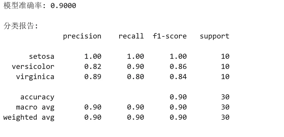
1 2 3 4 5 6 7 8 9 10 11 12 13 14 15 16 17 18 19 20 21 22 23 24 25 26 27 28 29 30 31 32 33 from sklearn.datasets import load_irisfrom sklearn.model_selection import train_test_splitfrom sklearn.preprocessing import StandardScalerfrom sklearn.ensemble import RandomForestClassifierfrom sklearn.metrics import accuracy_score, classification_report# ===== 完整的机器学习流程(5步)=====# 步骤1:加载数据iris = load_iris()X, y = iris.data, iris.target# 步骤2:划分数据X_train, X_test, y_train, y_test = train_test_split( X, y, test_size=0.2, random_state=42, stratify=y)# 步骤3:预处理scaler = StandardScaler()X_train_scaled = scaler.fit_transform(X_train)X_test_scaled = scaler.transform(X_test)# 步骤4:训练模型model = RandomForestClassifier(n_estimators=100, random_state=42)model.fit(X_train_scaled, y_train)# 步骤5:评估y_pred = model.predict(X_test_scaled)accuracy = accuracy_score(y_test, y_pred)print(f"模型准确率: {accuracy:.4f}")print("\n分类报告:")print(classification_report(y_test, y_pred, target_names=iris.target_names))
4.3 实战示例:三个典型机器学习任务
示例 1:分类任务 - 手写数字识别
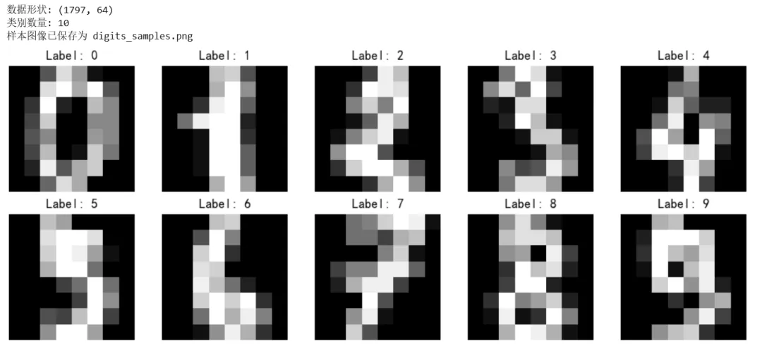
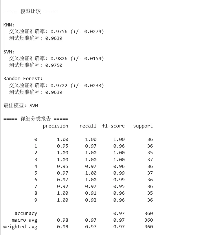
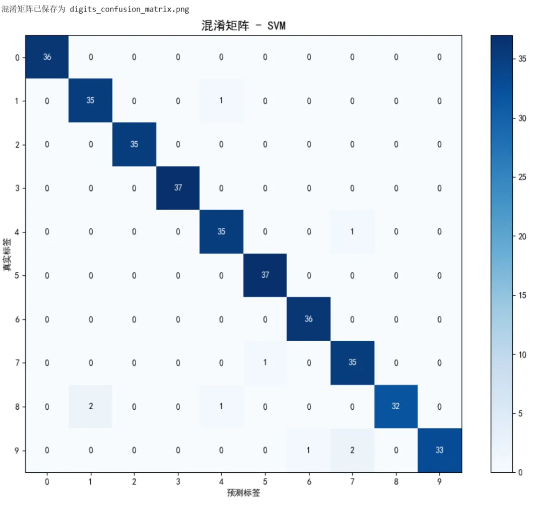
1 2 3 4 5 6 7 8 9 10 11 12 13 14 15 16 17 18 19 20 21 22 23 24 25 26 27 28 29 30 31 32 33 34 35 36 37 38 39 40 41 42 43 44 45 46 47 48 49 50 51 52 53 54 55 56 57 58 59 60 61 62 63 64 65 66 67 68 69 70 71 72 73 74 75 76 77 78 79 80 81 82 83 84 85 86 87 88 89 90 91 92 93 94 95 96 97 98 99 from sklearn.datasets import load_digitsfrom sklearn.model_selection import train_test_split, cross_val_scorefrom sklearn.preprocessing import StandardScalerfrom sklearn.neighbors import KNeighborsClassifierfrom sklearn.svm import SVCfrom sklearn.ensemble import RandomForestClassifierfrom sklearn.metrics import classification_report, confusion_matriximport matplotlib.pyplot as pltimport numpy as np# ===== 场景:手写数字识别 =====# 加载数据digits = load_digits()X, y = digits.data, digits.targetprint(f"数据形状: {X.shape}") # (1797, 64) - 8x8像素展平为64维向量print(f"类别数量: {len(digits.target_names)}") # 10个数字(0-9)# 可视化部分样本fig, axes = plt.subplots(2, 5, figsize=(10, 4))for i, ax in enumerate(axes.flat): ax.imshow(digits.images[i], cmap='gray') ax.set_title(f"Label: {digits.target[i]}") ax.axis('off')plt.tight_layout()plt.savefig('digits_samples.png', dpi=100)print("样本图像已保存为 digits_samples.png")plt.show()# 划分数据X_train, X_test, y_train, y_test = train_test_split( X, y, test_size=0.2, random_state=42, stratify=y)# 标准化scaler = StandardScaler()X_train_scaled = scaler.fit_transform(X_train)X_test_scaled = scaler.transform(X_test)# ===== 比较多个模型 =====models = { 'KNN': KNeighborsClassifier(n_neighbors=5), 'SVM': SVC(kernel='rbf', C=1.0), 'Random Forest': RandomForestClassifier(n_estimators=100, random_state=42)}print("\n===== 模型比较 =====")results = {}for name, model in models.items(): # 交叉验证 cv_scores = cross_val_score(model, X_train_scaled, y_train, cv=5) # 训练并在测试集评估 model.fit(X_train_scaled, y_train) test_score = model.score(X_test_scaled, y_test) results[name] = { 'cv_mean': cv_scores.mean(), 'cv_std': cv_scores.std(), 'test_accuracy': test_score } print(f"\n{name}:") print(f" 交叉验证准确率: {cv_scores.mean():.4f} (+/- {cv_scores.std()*2:.4f})") print(f" 测试集准确率: {test_score:.4f}")# 选择最佳模型(Random Forest 通常表现最好)best_model_name = max(results, key=lambda x: results[x]['test_accuracy'])best_model = models[best_model_name]print(f"\n最佳模型: {best_model_name}")# 详细评估y_pred = best_model.predict(X_test_scaled)print("\n===== 详细分类报告 =====")print(classification_report(y_test, y_pred))# 混淆矩阵可视化cm = confusion_matrix(y_test, y_pred)plt.figure(figsize=(10, 8))plt.imshow(cm, cmap='Blues')plt.title(f'混淆矩阵 - {best_model_name}', fontsize=14)plt.colorbar()plt.xlabel('预测标签')plt.ylabel('真实标签')plt.xticks(range(10))plt.yticks(range(10))# 添加数值for i in range(10): for j in range(10): plt.text(j, i, cm[i, j], ha='center', va='center', color='white' if cm[i, j] > cm.max()/2 else 'black')plt.tight_layout()plt.savefig('digits_confusion_matrix.png', dpi=150)print("混淆矩阵已保存为 digits_confusion_matrix.png")plt.show()
示例 2:回归任务 - 波士顿房价预测
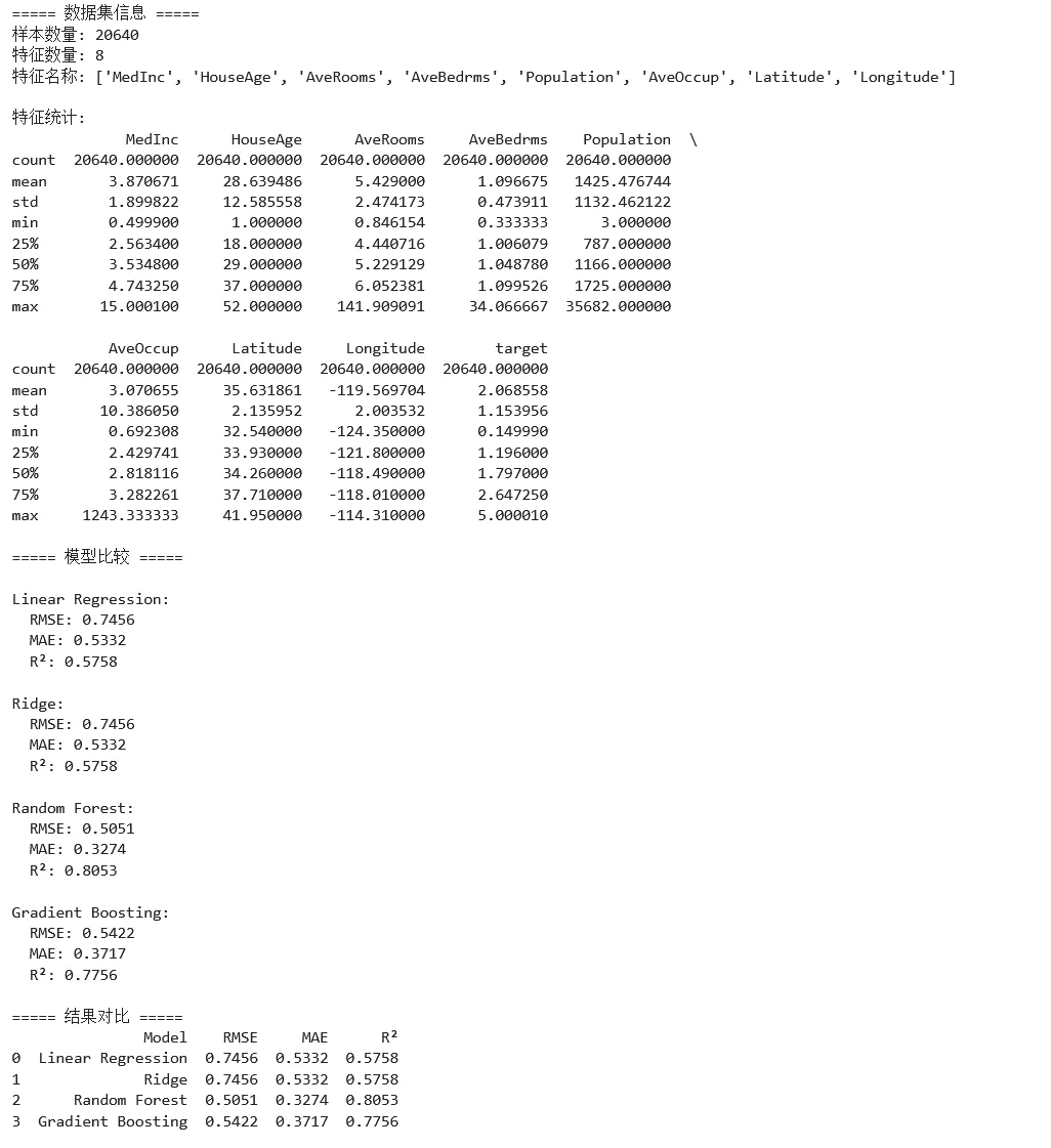
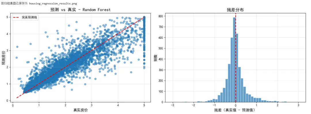
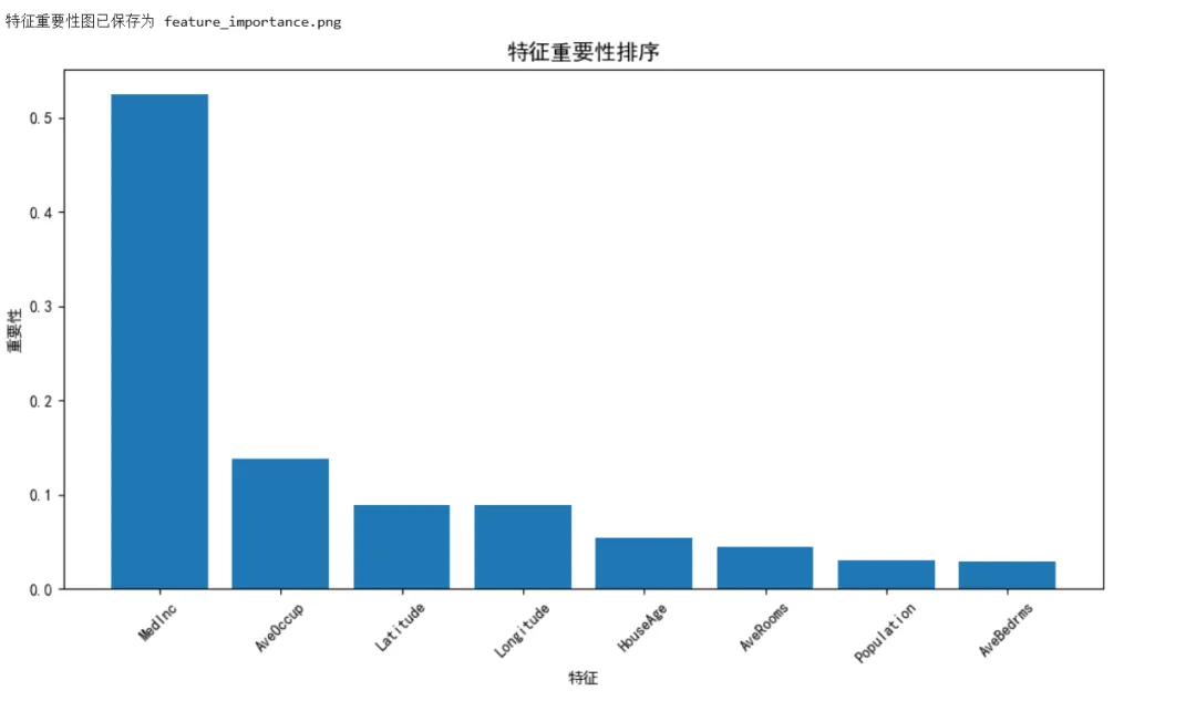
1 2 3 4 5 6 7 8 9 10 11 12 13 14 15 16 17 18 19 20 21 22 23 24 25 26 27 28 29 30 31 32 33 34 35 36 37 38 39 40 41 42 43 44 45 46 47 48 49 50 51 52 53 54 55 56 57 58 59 60 61 62 63 64 65 66 67 68 69 70 71 72 73 74 75 76 77 78 79 80 81 82 83 84 85 86 87 88 89 90 91 92 93 94 95 96 97 98 99 100 101 102 103 104 105 106 107 108 109 110 111 112 113 114 115 116 117 118 119 120 121 122 123 124 125 126 127 128 from sklearn.datasets import fetch_california_housingfrom sklearn.model_selection import train_test_split, cross_val_scorefrom sklearn.preprocessing import StandardScalerfrom sklearn.linear_model import LinearRegression, Ridge, Lassofrom sklearn.ensemble import RandomForestRegressor, GradientBoostingRegressorfrom sklearn.metrics import mean_squared_error, r2_score, mean_absolute_errorimport pandas as pdimport numpy as npimport matplotlib.pyplot as plt# ===== 场景:房价预测 =====# 加载加州房价数据集housing = fetch_california_housing()X, y = housing.data, housing.targetfeature_names = housing.feature_namesprint("===== 数据集信息 =====")print(f"样本数量: {X.shape[0]}")print(f"特征数量: {X.shape[1]}")print(f"特征名称: {feature_names}")# 创建 DataFrame 便于分析df = pd.DataFrame(X, columns=feature_names)df['target'] = yprint("\n特征统计:")print(df.describe())# 划分数据X_train, X_test, y_train, y_test = train_test_split( X, y, test_size=0.2, random_state=42)# 标准化scaler = StandardScaler()X_train_scaled = scaler.fit_transform(X_train)X_test_scaled = scaler.transform(X_test)# ===== 比较多个回归模型 =====models = { 'Linear Regression': LinearRegression(), 'Ridge': Ridge(alpha=1.0), 'Random Forest': RandomForestRegressor(n_estimators=100, random_state=42), 'Gradient Boosting': GradientBoostingRegressor(n_estimators=100, random_state=42)}print("\n===== 模型比较 =====")results = []for name, model in models.items(): # 训练 model.fit(X_train_scaled, y_train) # 预测 y_pred = model.predict(X_test_scaled) # 评估指标 mse = mean_squared_error(y_test, y_pred) rmse = np.sqrt(mse) mae = mean_absolute_error(y_test, y_pred) r2 = r2_score(y_test, y_pred) results.append({ 'Model': name, 'RMSE': rmse, 'MAE': mae, 'R²': r2 }) print(f"\n{name}:") print(f" RMSE: {rmse:.4f}") print(f" MAE: {mae:.4f}") print(f" R²: {r2:.4f}")# 结果对比表格results_df = pd.DataFrame(results)print("\n===== 结果对比 =====")print(results_df.round(4))# 选择最佳模型best_model_name = results_df.loc[results_df['R²'].idxmax(), 'Model']best_model = models[best_model_name]# ===== 可视化预测结果 =====y_pred = best_model.predict(X_test_scaled)fig, axes = plt.subplots(1, 2, figsize=(14, 5))# 子图1:预测值 vs 真实值axes[0].scatter(y_test, y_pred, alpha=0.5)axes[0].plot([y_test.min(), y_test.max()], [y_test.min(), y_test.max()], 'r--', linewidth=2, label='完美预测线')axes[0].set_xlabel('真实房价', fontsize=12)axes[0].set_ylabel('预测房价', fontsize=12)axes[0].set_title(f'预测 vs 真实 - {best_model_name}', fontsize=14)axes[0].legend()axes[0].grid(True, alpha=0.3)# 子图2:残差分布residuals = y_test - y_predaxes[1].hist(residuals, bins=50, edgecolor='white', alpha=0.7)axes[1].axvline(0, color='red', linestyle='--', linewidth=2)axes[1].set_xlabel('残差(真实值 - 预测值)', fontsize=12)axes[1].set_ylabel('频数', fontsize=12)axes[1].set_title('残差分布', fontsize=14)axes[1].grid(True, alpha=0.3)plt.tight_layout()plt.savefig('housing_regression_results.png', dpi=150)print("\n回归结果图已保存为 housing_regression_results.png")plt.show()# ===== 特征重要性 =====if hasattr(best_model, 'feature_importances_'): importances = best_model.feature_importances_ indices = np.argsort(importances)[::-1] plt.figure(figsize=(10, 6)) plt.title('特征重要性排序', fontsize=14) plt.bar(range(len(importances)), importances[indices], align='center') plt.xticks(range(len(importances)), [feature_names[i] for i in indices], rotation=45) plt.xlabel('特征') plt.ylabel('重要性') plt.tight_layout() plt.savefig('feature_importance.png', dpi=150) print("特征重要性图已保存为 feature_importance.png") plt.show()
示例 3:聚类与降维
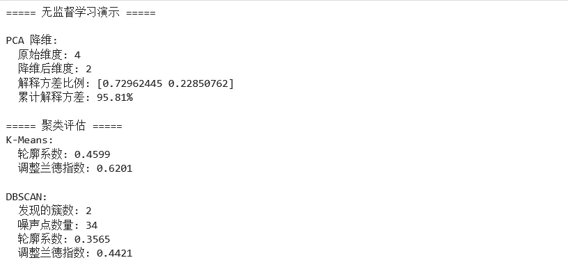
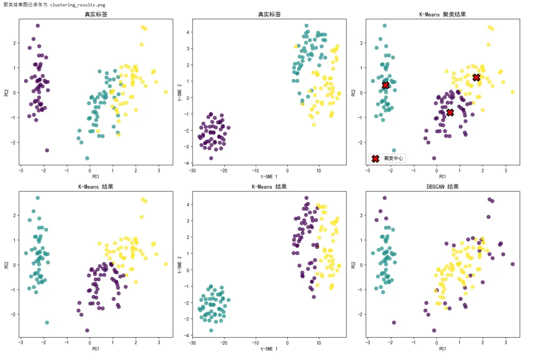
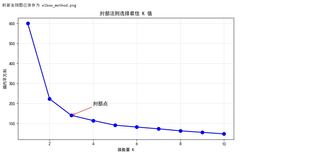
1 2 3 4 5 6 7 8 9 10 11 12 13 14 15 16 17 18 19 20 21 22 23 24 25 26 27 28 29 30 31 32 33 34 35 36 37 38 39 40 41 42 43 44 45 46 47 48 49 50 51 52 53 54 55 56 57 58 59 60 61 62 63 64 65 66 67 68 69 70 71 72 73 74 75 76 77 78 79 80 81 82 83 84 85 86 87 88 89 90 91 92 93 94 95 96 97 98 99 100 101 102 103 104 105 106 107 108 109 110 111 112 113 114 115 116 117 118 119 120 121 122 123 124 125 126 127 128 129 130 131 132 133 134 135 136 from sklearn.datasets import load_iris, make_blobsfrom sklearn.preprocessing import StandardScalerfrom sklearn.decomposition import PCAfrom sklearn.manifold import TSNEfrom sklearn.cluster import KMeans, DBSCANfrom sklearn.metrics import silhouette_score, adjusted_rand_scoreimport matplotlib.pyplot as pltimport numpy as np# ===== 场景:无监督学习 - 聚类与降维 =====# 加载鸢尾花数据(不使用标签)iris = load_iris()X = iris.datay_true = iris.target # 仅用于评估print("===== 无监督学习演示 =====")# 标准化scaler = StandardScaler()X_scaled = scaler.fit_transform(X)# ===== 降维 =====# PCA 降维pca = PCA(n_components=2)X_pca = pca.fit_transform(X_scaled)print(f"\nPCA 降维:")print(f" 原始维度: {X.shape[1]}")print(f" 降维后维度: {X_pca.shape[1]}")print(f" 解释方差比例: {pca.explained_variance_ratio_}")print(f" 累计解释方差: {sum(pca.explained_variance_ratio_):.2%}")# t-SNE 降维tsne = TSNE(n_components=2, random_state=42, perplexity=30)X_tsne = tsne.fit_transform(X_scaled)# ===== 聚类 =====# K-Meanskmeans = KMeans(n_clusters=3, random_state=42, n_init=10)labels_kmeans = kmeans.fit_predict(X_scaled)# DBSCANdbscan = DBSCAN(eps=0.5, min_samples=5)labels_dbscan = dbscan.fit_predict(X_scaled)# 评估聚类质量print("\n===== 聚类评估 =====")print("K-Means:")print(f" 轮廓系数: {silhouette_score(X_scaled, labels_kmeans):.4f}")print(f" 调整兰德指数: {adjusted_rand_score(y_true, labels_kmeans):.4f}")print("\nDBSCAN:")# DBSCAN 可能产生噪声点(标签=-1)n_clusters = len(set(labels_dbscan)) - (1 if -1 in labels_dbscan else 0)n_noise = list(labels_dbscan).count(-1)print(f" 发现的簇数: {n_clusters}")print(f" 噪声点数量: {n_noise}")if n_clusters > 1: print(f" 轮廓系数: {silhouette_score(X_scaled, labels_dbscan):.4f}")print(f" 调整兰德指数: {adjusted_rand_score(y_true, labels_dbscan):.4f}")# ===== 可视化 =====fig, axes = plt.subplots(2, 3, figsize=(15, 10))# 第一行:真实标签axes[0, 0].scatter(X_pca[:, 0], X_pca[:, 1], c=y_true, cmap='viridis', s=50, alpha=0.7)axes[0, 0].set_title('真实标签axes[0, 0].set_xlabel('PC1')axes[0, 0].set_ylabel('PC2')axes[0, 1].scatter(X_tsne[:, 0], X_tsne[:, 1], c=y_true, cmap='viridis', s=50, alpha=0.7)axes[0, 1].set_title('真实标签axes[0, 1].set_xlabel('t-SNE 1')axes[0, 1].set_ylabel('t-SNE 2')# 聚类中心可视化(K-Means + PCA)centers = kmeans.cluster_centers_centers_pca = pca.transform(centers)axes[0, 2].scatter(X_pca[:, 0], X_pca[:, 1], c=labels_kmeans, cmap='viridis', s=50, alpha=0.7)axes[0, 2].scatter(centers_pca[:, 0], centers_pca[:, 1], c='red', marker='X', s=200, edgecolors='black', linewidths=2, label='聚类中心')axes[0, 2].set_title('K-Means 聚类结果axes[0, 2].set_xlabel('PC1')axes[0, 2].set_ylabel('PC2')axes[0, 2].legend()# 第二行:K-Means 结果axes[1, 0].scatter(X_pca[:, 0], X_pca[:, 1], c=labels_kmeans, cmap='viridis', s=50, alpha=0.7)axes[1, 0].set_title('K-Means 结果axes[1, 0].set_xlabel('PC1')axes[1, 0].set_ylabel('PC2')axes[1, 1].scatter(X_tsne[:, 0], X_tsne[:, 1], c=labels_kmeans, cmap='viridis', s=50, alpha=0.7)axes[1, 1].set_title('K-Means 结果axes[1, 1].set_xlabel('t-SNE 1')axes[1, 1].set_ylabel('t-SNE 2')# DBSCAN 结果axes[1, 2].scatter(X_pca[:, 0], X_pca[:, 1], c=labels_dbscan, cmap='viridis', s=50, alpha=0.7)axes[1, 2].set_title('DBSCAN 结果axes[1, 2].set_xlabel('PC1')axes[1, 2].set_ylabel('PC2')plt.tight_layout()plt.savefig('clustering_results.png', dpi=150)print("\n聚类结果图已保存为 clustering_results.png")plt.show()# ===== K值选择:肘部法则 =====inertias = []K_range = range(1, 11)for k in K_range: kmeans = KMeans(n_clusters=k, random_state=42, n_init=10) kmeans.fit(X_scaled) inertias.append(kmeans.inertia_)plt.figure(figsize=(8, 5))plt.plot(K_range, inertias, 'bo-', linewidth=2, markersize=8)plt.xlabel('簇数量 K')plt.ylabel('簇内平方和plt.title('肘部法则选择最佳 K 值')plt.grid(True, alpha=0.3)# 标注肘部plt.annotate('肘部点', xy=(3, inertias[2]), xytext=(4, inertias[2]+50), fontsize=12, arrowprops=dict(arrowstyle='->', color='red'))plt.tight_layout()plt.savefig('elbow_method.png', dpi=150)print("肘部法则图已保存为 elbow_method.png")plt.show()
4.4 Pipeline 与超参数调优
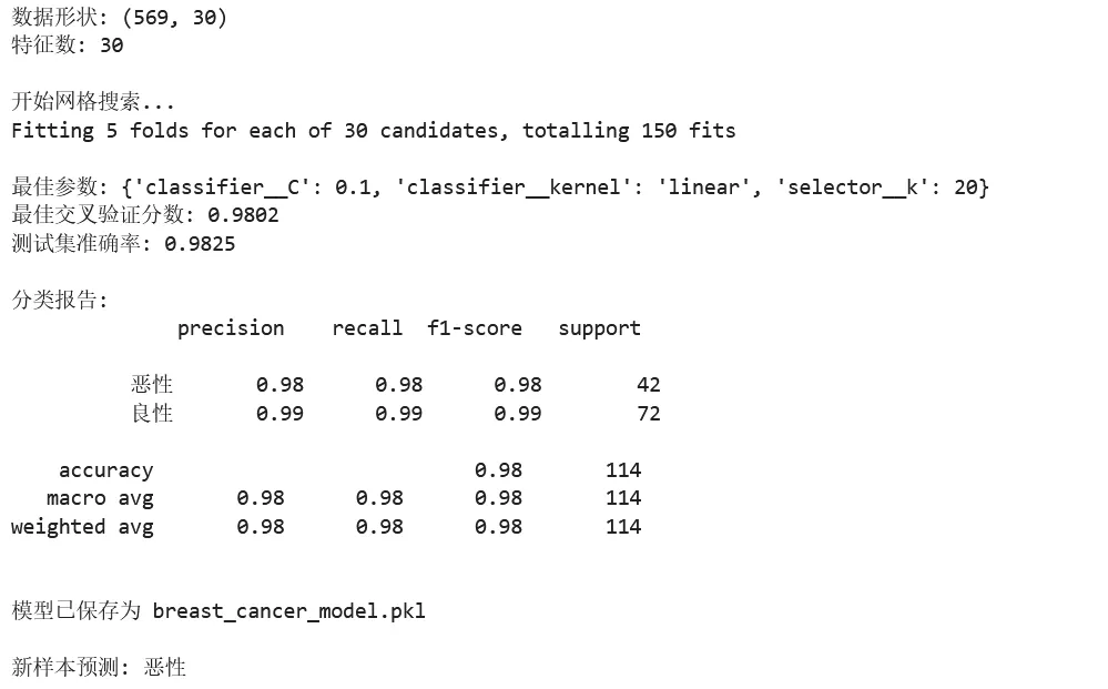
1 2 3 4 5 6 7 8 9 10 11 12 13 14 15 16 17 18 19 20 21 22 23 24 25 26 27 28 29 30 31 32 33 34 35 36 37 38 39 40 41 42 43 44 45 46 47 48 49 50 51 52 53 54 55 56 57 58 59 60 61 62 63 64 65 66 67 68 69 70 71 72 73 74 75 76 77 78 79 80 81 82 83 84 from sklearn.datasets import load_breast_cancerfrom sklearn.model_selection import train_test_split, GridSearchCV, cross_val_scorefrom sklearn.preprocessing import StandardScalerfrom sklearn.feature_selection import SelectKBest, f_classiffrom sklearn.svm import SVCfrom sklearn.pipeline import Pipelinefrom sklearn.metrics import classification_reportimport numpy as np# ===== 场景:完整的机器学习管道 =====# 加载数据data = load_breast_cancer()X, y = data.data, data.targetprint(f"数据形状: {X.shape}") # (569, 30)print(f"特征数: {X.shape[1]}")# 划分数据X_train, X_test, y_train, y_test = train_test_split( X, y, test_size=0.2, random_state=42, stratify=y)# ===== 创建 Pipeline =====# Pipeline 将预处理和模型训练串联起来# 好处:避免数据泄露,代码更简洁pipeline = Pipeline([ ('scaler', StandardScaler()), # 步骤1:标准化 ('selector', SelectKBest(f_classif)), # 步骤2:特征选择 ('classifier', SVC()) # 步骤3:分类器])# ===== 超参数网格搜索 =====# 定义参数网格param_grid = { 'selector__k': [5, 10, 15, 20, 'all'], # 选择多少个特征 'classifier__C': [0.1, 1, 10], # SVM 正则化参数 'classifier__kernel': ['rbf', 'linear'] # SVM 核函数}# 网格搜索grid_search = GridSearchCV( pipeline, param_grid, cv=5, # 5折交叉验证 scoring='accuracy', n_jobs=-1, # 使用所有 CPU 核心 verbose=1 # 显示进度)print("\n开始网格搜索...")grid_search.fit(X_train, y_train)# 输出最佳参数print(f"\n最佳参数: {grid_search.best_params_}")print(f"最佳交叉验证分数: {grid_search.best_score_:.4f}")# 在测试集上评估best_model = grid_search.best_estimator_test_score = best_model.score(X_test, y_test)print(f"测试集准确率: {test_score:.4f}")# 详细评估报告y_pred = best_model.predict(X_test)print("\n分类报告:")print(classification_report(y_test, y_pred, target_names=['恶性', '良性']))# ===== 模型持久化 =====import joblib# 保存模型joblib.dump(best_model, 'breast_cancer_model.pkl')print("\n模型已保存为 breast_cancer_model.pkl")# 加载模型loaded_model = joblib.load('breast_cancer_model.pkl')# 预测新样本(模拟)new_sample = X_test[:1] # 取第一个测试样本prediction = loaded_model.predict(new_sample)print(f"\n新样本预测: {'恶性' if prediction[0] == 0 else '良性'}")
4.5 Scikit-learn 常用功能速查表
数据预处理
StandardScaler | with_mean, with_std | |
MinMaxScaler | feature_range | |
Normalizer | norm | |
LabelEncoder | ||
OneHotEncoder | sparse, handle_unknown | |
PolynomialFeatures | degree, interaction_only |
特征选择
SelectKBest | score_func, k | |
SelectPercentile | score_func, percentile | |
RFE | estimator, n_features_to_select |
分类算法
LogisticRegression | C, penalty, solver | |
KNeighborsClassifier | n_neighbors, weights | |
SVC | C, kernel, gamma | |
DecisionTreeClassifier | max_depth, min_samples_split | |
RandomForestClassifier | n_estimators, max_depth | |
GradientBoostingClassifier | n_estimators, learning_rate |
回归算法
LinearRegression | ||
Ridge | alpha | |
Lasso | alpha | |
RandomForestRegressor | n_estimators, max_depth |
聚类算法
KMeans | n_clusters, n_init | |
DBSCAN | eps, min_samples | |
AgglomerativeClustering | n_clusters, linkage |
降维算法
PCA | n_components | |
TruncatedSVD | n_components | |
TSNE | n_components, perplexity |
模型评估
accuracy_score | ||
precision_score | ||
recall_score | ||
f1_score | ||
roc_auc_score | ||
mean_squared_error | ||
r2_score | ||
silhouette_score |
第五章:房价预测完整项目
5.1 项目概述
目标:预测加利福尼亚州各区域的房价中位数
数据流程:
1 2 原始数据 → Pandas(清洗与特征工程)→ NumPy(数值转换)→ Matplotlib(可视化分析)→ Scikit-learn(建模与评估)
5.2 完整代码实现
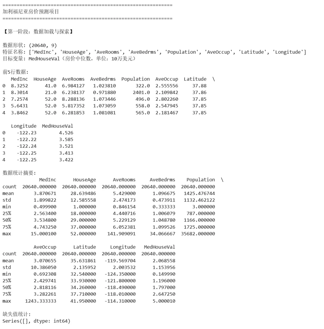
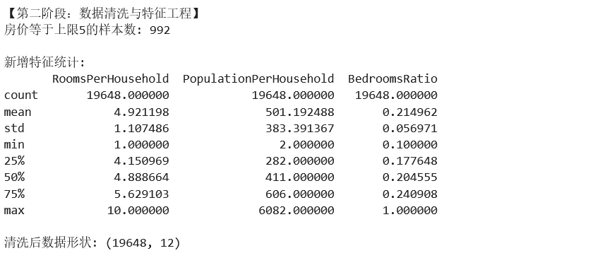
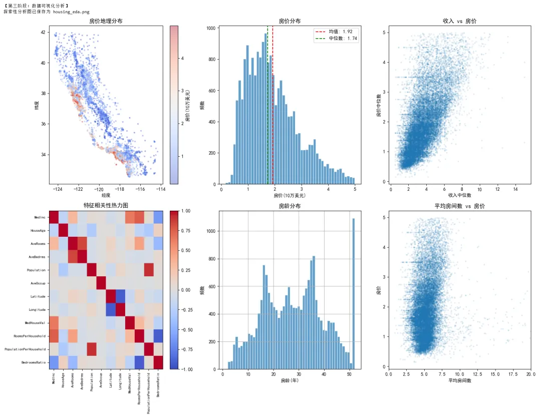
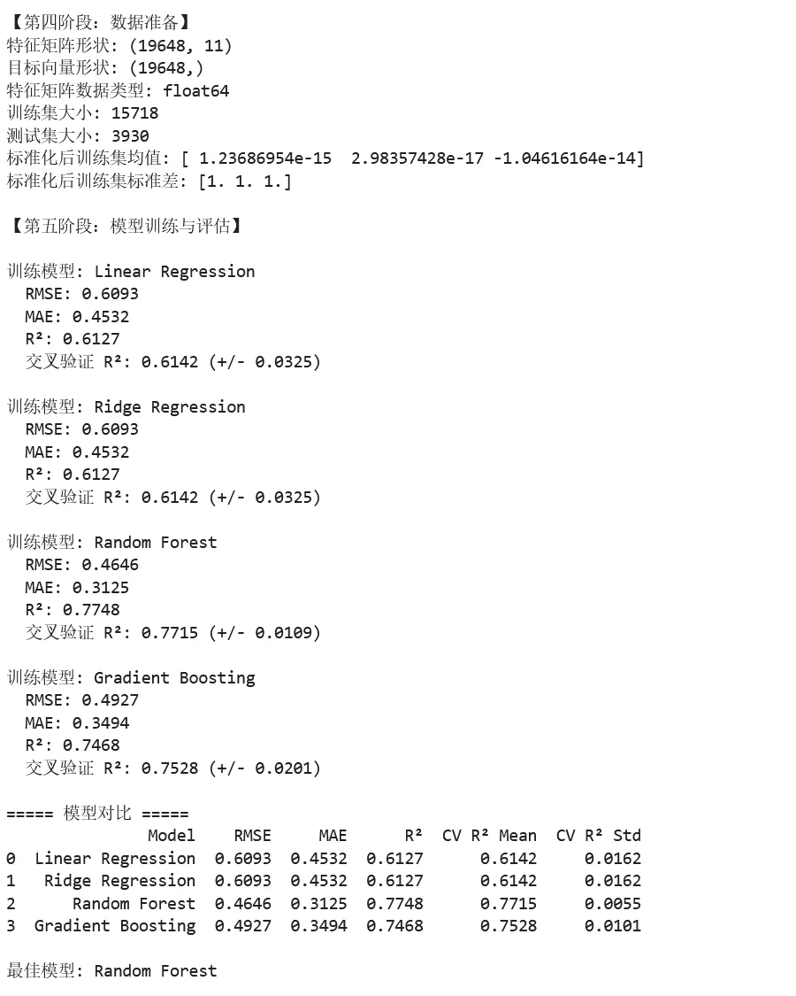
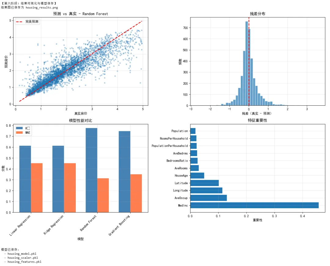
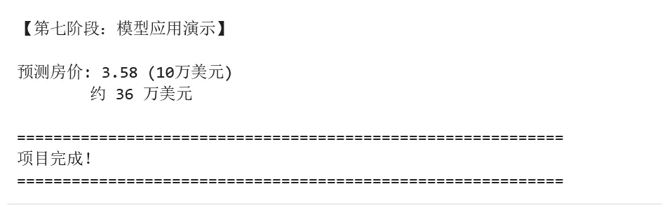
1 2 3 4 5 6 7 8 9 10 11 12 13 14 15 16 17 18 19 20 21 22 23 24 25 26 27 28 29 30 31 32 33 34 35 36 37 38 39 40 41 42 43 44 45 46 47 48 49 50 51 52 53 54 55 56 57 58 59 60 61 62 63 64 65 66 67 68 69 70 71 72 73 74 75 76 77 78 79 80 81 82 83 84 85 86 87 88 89 90 91 92 93 94 95 96 97 98 99 100 101 102 103 104 105 106 107 108 109 110 111 112 113 114 115 116 117 118 119 120 121 122 123 124 125 126 127 128 129 130 131 132 133 134 135 136 137 138 139 140 141 142 143 144 145 146 147 148 149 150 151 152 153 154 155 156 157 158 159 160 161 162 163 164 165 166 167 168 169 170 171 172 173 174 175 176 177 178 179 180 181 182 183 184 185 186 187 188 189 190 191 192 193 194 195 196 197 198 199 200 201 202 203 204 205 206 207 208 209 210 211 212 213 214 215 216 217 218 219 220 221 222 223 224 225 226 227 228 229 230 231 232 233 234 235 236 237 238 239 240 241 242 243 244 245 246 247 248 249 250 251 252 253 254 255 256 257 258 259 260 261 262 263 264 265 266 267 268 269 270 271 272 273 274 275 276 277 278 279 280 281 282 283 284 285 286 287 288 289 290 291 292 293 294 295 296 297 298 299 300 301 302 303 304 305 306 307 308 309 310 311 312 313 314 315 316 317 318 319 320 321 322 323 324 325 326 327 328 329 330 331 332 333 334 335 336 337 338 339 340 341 342 343 344 345 346 347 348 349 350 351 352 353 354 355 356 357 358 359 360 361 362 363 364 365 366 367 368 369 370 371 372 # =================================================================# 项目:加利福尼亚房价预测# 技术栈:NumPy + Pandas + Matplotlib + Scikit-learn# =================================================================import numpy as npimport pandas as pdimport matplotlib.pyplot as pltimport seaborn as snsfrom sklearn.datasets import fetch_california_housingfrom sklearn.model_selection import train_test_split, cross_val_score, GridSearchCVfrom sklearn.preprocessing import StandardScalerfrom sklearn.linear_model import LinearRegression, Ridge, Lassofrom sklearn.ensemble import RandomForestRegressor, GradientBoostingRegressorfrom sklearn.metrics import mean_squared_error, r2_score, mean_absolute_errorimport joblibimport warningswarnings.filterwarnings('ignore')# 设置中文显示plt.rcParams['font.sans-serif'] = ['SimHei', 'Arial Unicode MS']plt.rcParams['axes.unicode_minus'] = Falseprint("=" * 60)print("加利福尼亚房价预测项目")print("=" * 60)# =================================================================# 第一阶段:数据加载与探索(Pandas + NumPy)# =================================================================print("\n【第一阶段:数据加载与探索】")# 加载数据housing = fetch_california_housing(as_frame=True)df = housing.frameprint(f"\n数据形状: {df.shape}")print(f"特征名称: {housing.feature_names}")print(f"目标变量: MedHouseVal(房价中位数,单位:10万美元)")# 数据概览print("\n前5行数据:")print(df.head())print("\n数据统计摘要:")print(df.describe())# 检查缺失值missing = df.isnull().sum()print(f"\n缺失值统计:\n{missing[missing > 0]}")# =================================================================# 第二阶段:数据清洗与特征工程# =================================================================print("\n【第二阶段:数据清洗与特征工程】")# 创建特征副本df_clean = df.copy()# 1. 处理异常值# 房价上限为5(数据被截断),移除这些样本print(f"房价等于上限5的样本数: {(df_clean['MedHouseVal'] >= 5.0).sum()}")df_clean = df_clean[df_clean['MedHouseVal'] < 5.0]# 2. 特征工程# 添加新特征:每户房间数df_clean['RoomsPerHousehold'] = df_clean['AveRooms'] / df_clean['AveBedrms']# 每人房间数df_clean['PopulationPerHousehold'] = df_clean['Population'] / df_clean['AveOccup']# 卧室占比df_clean['BedroomsRatio'] = df_clean['AveBedrms'] / df_clean['AveRooms']print("\n新增特征统计:")print(df_clean[['RoomsPerHousehold', 'PopulationPerHousehold', 'BedroomsRatio']].describe())# 处理无穷大值(除以接近0的数导致)df_clean = df_clean.replace([np.inf, -np.inf], np.nan).dropna()print(f"\n清洗后数据形状: {df_clean.shape}")# =================================================================# 第三阶段:数据可视化分析# =================================================================print("\n【第三阶段:数据可视化分析】")# 创建多子图fig = plt.figure(figsize=(16, 12))# 子图1:房价地理分布ax1 = fig.add_subplot(2, 3, 1)scatter = ax1.scatter(df_clean['Longitude'], df_clean['Latitude'], c=df_clean['MedHouseVal'], cmap='coolwarm', alpha=0.4, s=5)ax1.set_title('房价地理分布')ax1.set_xlabel('经度')ax1.set_ylabel('纬度')plt.colorbar(scatter, ax=ax1, label='房价(10万美元)')# 子图2:房价分布直方图ax2 = fig.add_subplot(2, 3, 2)ax2.hist(df_clean['MedHouseVal'], bins=50, edgecolor='white', alpha=0.7)ax2.axvline(df_clean['MedHouseVal'].mean(), color='red', linestyle='--', label=f'均值: {df_clean["MedHouseVal"].mean():.2f}')ax2.axvline(df_clean['MedHouseVal'].median(), color='green', linestyle='--', label=f'中位数: {df_clean["MedHouseVal"].median():.2f}')ax2.set_title('房价分布')ax2.set_xlabel('房价(10万美元)')ax2.set_ylabel('频数')ax2.legend()# 子图3:收入与房价关系ax3 = fig.add_subplot(2, 3, 3)ax3.scatter(df_clean['MedInc'], df_clean['MedHouseVal'], alpha=0.1, s=5)ax3.set_title('收入 vs 房价')ax3.set_xlabel('收入中位数')ax3.set_ylabel('房价中位数')# 子图4:相关性热力图ax4 = fig.add_subplot(2, 3, 4)correlation = df_clean.corr()im = ax4.imshow(correlation, cmap='coolwarm', aspect='auto', vmin=-1, vmax=1)ax4.set_title('特征相关性热力图')ax4.set_xticks(range(len(correlation.columns)))ax4.set_yticks(range(len(correlation.columns)))ax4.set_xticklabels(correlation.columns, rotation=90, fontsize=8)ax4.set_yticklabels(correlation.columns, fontsize=8)plt.colorbar(im, ax=ax4)# 子图5:房龄分布ax5 = fig.add_subplot(2, 3, 5)df_clean['HouseAge'].hist(bins=52, ax=ax5, edgecolor='white', alpha=0.7)ax5.set_title('房龄分布')ax5.set_xlabel('房龄(年)')ax5.set_ylabel('频数')# 子图6:房间数与房价ax6 = fig.add_subplot(2, 3, 6)ax6.scatter(df_clean['AveRooms'], df_clean['MedHouseVal'], alpha=0.1, s=5)ax6.set_xlim(0, 20) # 限制x轴范围,排除极端值ax6.set_title('平均房间数 vs 房价')ax6.set_xlabel('平均房间数')ax6.set_ylabel('房价')plt.tight_layout()plt.savefig('housing_eda.png', dpi=150, bbox_inches='tight')print("探索性分析图已保存为 housing_eda.png")plt.show()# =================================================================# 第四阶段:数据准备# =================================================================print("\n【第四阶段:数据准备】")# 分离特征和目标feature_cols = [col for col in df_clean.columns if col != 'MedHouseVal']X = df_clean[feature_cols]y = df_clean['MedHouseVal']# NumPy 数组转换(sklearn 内部会自动做,但理解这个过程很重要)X_array = X.values # DataFrame → NumPy arrayy_array = y.valuesprint(f"特征矩阵形状: {X_array.shape}")print(f"目标向量形状: {y_array.shape}")print(f"特征矩阵数据类型: {X_array.dtype}")# 划分训练集和测试集X_train, X_test, y_train, y_test = train_test_split( X_array, y_array, test_size=0.2, random_state=42)print(f"训练集大小: {X_train.shape[0]}")print(f"测试集大小: {X_test.shape[0]}")# 标准化scaler = StandardScaler()X_train_scaled = scaler.fit_transform(X_train)X_test_scaled = scaler.transform(X_test)print(f"标准化后训练集均值: {X_train_scaled.mean(axis=0)[:3]}") # 应该接近0print(f"标准化后训练集标准差: {X_train_scaled.std(axis=0)[:3]}") # 应该接近1# =================================================================# 第五阶段:模型训练与评估# =================================================================print("\n【第五阶段:模型训练与评估】")# 定义多个模型models = { 'Linear Regression': LinearRegression(), 'Ridge Regression': Ridge(alpha=1.0), 'Random Forest': RandomForestRegressor(n_estimators=100, random_state=42, n_jobs=-1), 'Gradient Boosting': GradientBoostingRegressor(n_estimators=100, random_state=42)}# 训练和评估results = []for name, model in models.items(): print(f"\n训练模型: {name}") # 训练 model.fit(X_train_scaled, y_train) # 预测 y_pred = model.predict(X_test_scaled) # 评估指标 mse = mean_squared_error(y_test, y_pred) rmse = np.sqrt(mse) mae = mean_absolute_error(y_test, y_pred) r2 = r2_score(y_test, y_pred) # 交叉验证 cv_scores = cross_val_score(model, X_train_scaled, y_train, cv=5, scoring='r2') results.append({ 'Model': name, 'RMSE': rmse, 'MAE': mae, 'R²': r2, 'CV R² Mean': cv_scores.mean(), 'CV R² Std': cv_scores.std() }) print(f" RMSE: {rmse:.4f}") print(f" MAE: {mae:.4f}") print(f" R²: {r2:.4f}") print(f" 交叉验证 R²: {cv_scores.mean():.4f} (+/- {cv_scores.std()*2:.4f})")# 结果对比results_df = pd.DataFrame(results)print("\n===== 模型对比 =====")print(results_df.round(4))# 选择最佳模型best_idx = results_df['R²'].idxmax()best_model_name = results_df.loc[best_idx, 'Model']best_model = models[best_model_name]print(f"\n最佳模型: {best_model_name}")# =================================================================# 第六阶段:结果可视化与模型保存# =================================================================print("\n【第六阶段:结果可视化与模型保存】")# 重新预测最佳模型y_pred = best_model.predict(X_test_scaled)# 创建结果可视化fig, axes = plt.subplots(2, 2, figsize=(14, 10))# 子图1:预测值 vs 真实值axes[0, 0].scatter(y_test, y_pred, alpha=0.3, s=10)axes[0, 0].plot([y_test.min(), y_test.max()], [y_test.min(), y_test.max()], 'r--', linewidth=2, label='完美预测')axes[0, 0].set_xlabel('真实房价')axes[0, 0].set_ylabel('预测房价')axes[0, 0].set_title(f'预测 vs 真实 - {best_model_name}')axes[0, 0].legend()axes[0, 0].grid(True, alpha=0.3)# 子图2:残差分布residuals = y_test - y_predaxes[0, 1].hist(residuals, bins=50, edgecolor='white', alpha=0.7)axes[0, 1].axvline(0, color='red', linestyle='--', linewidth=2)axes[0, 1].set_xlabel('残差(真实 - 预测)')axes[0, 1].set_ylabel('频数')axes[0, 1].set_title('残差分布')axes[0, 1].grid(True, alpha=0.3)# 子图3:模型对比柱状图x_pos = np.arange(len(results_df))width = 0.35axes[1, 0].bar(x_pos - width/2, results_df['R²'], width, label='R²', color='steelblue')axes[1, 0].bar(x_pos + width/2, results_df['MAE'], width, label='MAE', color='coral')axes[1, 0].set_xlabel('模型')axes[1, 0].set_ylabel('分数')axes[1, 0].set_title('模型性能对比')axes[1, 0].set_xticks(x_pos)axes[1, 0].set_xticklabels(results_df['Model'], rotation=45, ha='right')axes[1, 0].legend()axes[1, 0].grid(True, alpha=0.3)# 子图4:特征重要性(如果有)if hasattr(best_model, 'feature_importances_'): importances = best_model.feature_importances_ indices = np.argsort(importances)[::-1] axes[1, 1].barh(range(len(importances)), importances[indices], align='center') axes[1, 1].set_yticks(range(len(importances))) axes[1, 1].set_yticklabels([feature_cols[i] for i in indices]) axes[1, 1].set_xlabel('重要性') axes[1, 1].set_title('特征重要性') axes[1, 1].grid(True, alpha=0.3)else: # 如果模型没有feature_importances_,显示系数 if hasattr(best_model, 'coef_'): coef = np.abs(best_model.coef_) indices = np.argsort(coef)[::-1] axes[1, 1].barh(range(len(coef)), coef[indices], align='center') axes[1, 1].set_yticks(range(len(coef))) axes[1, 1].set_yticklabels([feature_cols[i] for i in indices]) axes[1, 1].set_xlabel('系数绝对值') axes[1, 1].set_title('特征重要性(系数绝对值)') axes[1, 1].grid(True, alpha=0.3) else: axes[1, 1].text(0.5, 0.5, '该模型不支持特征重要性', ha='center', va='center', fontsize=14) axes[1, 1].set_title('特征重要性')plt.tight_layout()plt.savefig('housing_results.png', dpi=150, bbox_inches='tight')print("结果图已保存为 housing_results.png")plt.show()# 保存模型joblib.dump(best_model, 'housing_model.pkl')joblib.dump(scaler, 'housing_scaler.pkl')joblib.dump(feature_cols, 'housing_features.pkl')print("\n模型已保存:")print(" - housing_model.pkl")print(" - housing_scaler.pkl")print(" - housing_features.pkl")# =================================================================# 第七阶段:模型应用演示# =================================================================print("\n【第七阶段:模型应用演示】")# 加载模型loaded_model = joblib.load('housing_model.pkl')loaded_scaler = joblib.load('housing_scaler.pkl')loaded_features = joblib.load('housing_features.pkl')# 模拟新数据(某个区域的特征)new_data = pd.DataFrame({ 'MedInc': [8.0], # 收入中位数较高 'HouseAge': [20], # 房龄20年 'AveRooms': [8.0], # 平均8个房间 'AveBedrms': [2.0], # 平均2个卧室 'Population': [1000], # 人口 'AveOccup': [3.0], # 平均住户 'Latitude': [34.0], # 纬度 'Longitude': [-118.0], # 经度 'RoomsPerHousehold': [8.0/2.0], 'PopulationPerHousehold': [1000/3.0], 'BedroomsRatio': [2.0/8.0]})# 确保特征顺序一致new_data = new_data[loaded_features]# 标准化new_data_scaled = loaded_scaler.transform(new_data.values)# 预测prediction = loaded_model.predict(new_data_scaled)print(f"\n预测房价: {prediction[0]:.2f} (10万美元)")print(f" 约 {prediction[0] * 10:.0f} 万美元")print("\n" + "=" * 60)print("项目完成!")print("=" * 60)
第六章:避坑指南
6.1 NumPy
✅ 推荐做法
1 2 3 4 5 6 7 8 9 10 11 12 13 14 15 16 17 18 19 20 21 22 23 24 25 26 27 28 import numpy as np# ✅ 1. 使用向量化操作代替循环# 好的做法arr = np.array([1, 2, 3, 4, 5])result = arr * 2 # 向量化乘法# ✅ 2. 预分配数组大小# 好的做法result = np.zeros(1000)for i in range(1000): result[i] = i ** 2# ✅ 3. 使用合适的数据类型# 好的做法:根据数据范围选择类型small_integers = np.array([1, 2, 3], dtype=np.int8) # 节省内存large_floats = np.array([1e10, 2e10], dtype=np.float64) # 精度要求高# ✅ 4. 使用广播机制# 好的做法matrix = np.random.rand(100, 5)row_means = matrix.mean(axis=1, keepdims=True) # 保持维度以便广播normalized = matrix - row_means# ✅ 5. 使用 np.where 进行条件选择# 好的做法arr = np.array([1, -2, 3, -4, 5])positive = np.where(arr > 0, arr, 0) # 将负数替换为0
❌ 避免的做法
1 2 3 4 5 6 7 8 9 10 11 12 13 14 15 16 17 18 19 20 21 22 23 24 25 26 27 28 29 30 31 32 33 34 35 36 37 import numpy as np# ❌ 1. 在循环中不断扩展数组# 不好的做法result = np.array([])for i in range(1000): result = np.append(result, i ** 2) # 每次都创建新数组,效率低# ❌ 2. 使用 Python 列表存储数值计算结果# 不好的做法result = []for i in range(1000): result.append(i ** 2)result = np.array(result) # 应该直接用 NumPy# ❌ 3. 忽略数据类型# 不好的做法arr = np.array([1, 2, 3]) # 默认int64,可能浪费内存# 如果确定数值范围小:arr = np.array([1, 2, 3], dtype=np.int8)# ❌ 4. 不必要地复制数组# 不好的做法large_arr = np.random.rand(10000, 10000)copy_arr = large_arr.copy() # 如果不需要修改,没必要复制result = copy_arr.sum() # 可以直接用 large_arr.sum()# ❌ 5. 使用 Python 循环处理 NumPy 数组# 不好的做法arr = np.array([1, 2, 3, 4, 5])result = []for x in arr: result.append(x ** 2)result = np.array(result)# 好的做法result = arr ** 2 # 直接向量化
6.2 Pandas
✅ 推荐做法
1 2 3 4 5 6 7 8 9 10 11 12 13 14 15 16 17 18 19 20 21 22 23 24 25 26 27 28 29 30 31 32 33 34 35 36 37 38 import pandas as pdimport numpy as np# ✅ 1. 使用 .loc 和 .iloc 明确索引方式df = pd.DataFrame({'A': [1, 2, 3], 'B': [4, 5, 6]})# 好的做法:明确的标签索引value = df.loc[0, 'A']# ✅ 2. 链式操作时使用 .copy() 避免警告# 好的做法df_subset = df[['A', 'B']].copy()df_subset['C'] = df_subset['A'] + df_subset['B']# ✅ 3. 使用 .isin() 进行多值筛选# 好的做法cities = ['New York', 'London', 'Tokyo']df_filtered = df[df['city'].isin(cities)]# ✅ 4. 使用 .agg() 进行多种聚合# 好的做法summary = df.groupby('category').agg({ 'price': ['mean', 'std', 'count'], 'quantity': 'sum'})# ✅ 5. 使用 pd.to_datetime 处理日期# 好的做法df['date'] = pd.to_datetime(df['date'], format='%Y-%m-%d', errors='coerce')# ✅ 6. 使用 .merge() 时指定后缀# 好的做法result = pd.merge(df1, df2, on='id', suffixes=('_left', '_right'))# ✅ 7. 使用 .astype() 优化内存# 好的做法df['category'] = df['category'].astype('category') # 分类数据df['small_int'] = df['small_int'].astype('int8') # 小整数
❌ 避免的做法
1 2 3 4 5 6 7 8 9 10 11 12 13 14 15 16 17 18 19 20 21 22 23 24 25 26 27 28 29 30 31 32 33 34 35 36 37 38 39 40 41 42 43 44 import pandas as pd# ❌ 1. 链式索引(导致 SettingWithCopyWarning)df = pd.DataFrame({'A': [1, 2, 3], 'B': [4, 5, 6]})# 不好的做法:链式索引df[df['A'] > 1]['B'] = 10 # 可能不会生效,且会产生警告# 好的做法:使用 .locdf.loc[df['A'] > 1, 'B'] = 10# ❌ 2. 在循环中逐行处理# 不好的做法for i in range(len(df)): df.loc[i, 'new_col'] = df.loc[i, 'A'] * 2# 好的做法:向量化操作df['new_col'] = df['A'] * 2# ❌ 3. 使用 append 逐行添加数据# 不好的做法result = pd.DataFrame()for i in range(1000): result = result.append({'a': i}, ignore_index=True) # 效率极低# 好的做法:先收集再创建data_list = []for i in range(1000): data_list.append({'a': i})result = pd.DataFrame(data_list)# ❌ 4. 忽略数据类型,浪费内存# 不好的做法:大量重复字符串df['status'] = ['active'] * 1000000 # 每个字符串单独存储# 好的做法:使用 category 类型df['status'] = pd.Categorical(['active'] * 1000000)# ❌ 5. 不指定列名读取数据# 不好的做法df = pd.read_csv('data.csv', header=None) # 列名是0, 1, 2...# 好的做法df = pd.read_csv('data.csv', names=['col1', 'col2', 'col3'])
6.3 Matplotlib
✅ 推荐做法
1 2 3 4 5 6 7 8 9 10 11 12 13 14 15 16 17 18 19 20 21 22 23 24 25 26 27 28 import matplotlib.pyplot as pltimport numpy as np# ✅ 1. 使用面向对象 API# 好的做法fig, ax = plt.subplots(figsize=(10, 6))ax.plot([1, 2, 3], [1, 4, 2])ax.set_xlabel('X轴')ax.set_title('标题')# ✅ 2. 保存时设置 DPI 和 bbox_inches# 好的做法fig.savefig('plot.png', dpi=150, bbox_inches='tight')# ✅ 3. 使用 plt.tight_layout() 避免重叠# 好的做法fig, axes = plt.subplots(2, 2)# ... 绑图 ...plt.tight_layout() # 自动调整子图间距# ✅ 4. 使用样式表统一风格# 好的做法plt.style.use('seaborn-v0_8-whitegrid') # 使用预设样式# ✅ 5. 中文显示正确设置# 好的做法plt.rcParams['font.sans-serif'] = ['SimHei', 'Arial Unicode MS']plt.rcParams['axes.unicode_minus'] = False
❌ 避免的做法
1 2 3 4 5 6 7 8 9 10 11 12 13 14 15 16 17 18 19 20 21 22 23 24 25 26 27 28 29 30 31 32 33 34 35 36 import matplotlib.pyplot as plt# ❌ 1. 在循环中重复创建 figure# 不好的做法for i in range(10): plt.figure() # 每次创建新 figure plt.plot([1, 2, 3]) plt.show()# 应该创建子图或关闭之前的 figure# ❌ 2. 忘记关闭图形(内存泄漏)# 不好的做法for i in range(100): fig = plt.figure() # ... 绑图 ... plt.savefig(f'plot_{i}.png') # 忘记 plt.close(fig)# 好的做法for i in range(100): fig = plt.figure() # ... 绑图 ... plt.savefig(f'plot_{i}.png') plt.close(fig) # 释放内存# ❌ 3. 使用 pyplot 接口处理复杂图形# 不好的做法:难以精确控制plt.subplot(2, 2, 1)plt.plot([1, 2, 3])plt.subplot(2, 2, 2)# ... 混乱# 好的做法:面向对象fig, axes = plt.subplots(2, 2)axes[0, 0].plot([1, 2, 3])axes[0, 1].plot([3, 2, 1])
6.4 Scikit-learn
✅ 推荐做法
1 2 3 4 5 6 7 8 9 10 11 12 13 14 15 16 17 18 19 20 21 22 23 24 25 26 27 28 29 30 31 32 33 34 35 36 37 from sklearn.model_selection import train_test_split, cross_val_scorefrom sklearn.preprocessing import StandardScalerfrom sklearn.ensemble import RandomForestClassifierfrom sklearn.pipeline import Pipelineimport joblib# ✅ 1. 始终划分训练集和测试集X_train, X_test, y_train, y_test = train_test_split( X, y, test_size=0.2, random_state=42, stratify=y)# ✅ 2. 使用 Pipeline 避免数据泄露# 好的做法pipeline = Pipeline([ ('scaler', StandardScaler()), ('classifier', RandomForestClassifier())])pipeline.fit(X_train, y_train)# ✅ 3. 使用交叉验证评估模型# 好的做法cv_scores = cross_val_score(model, X_train, y_train, cv=5)# ✅ 4. 标准化只在训练集上 fit# 好的做法scaler = StandardScaler()X_train_scaled = scaler.fit_transform(X_train) # fit_transformX_test_scaled = scaler.transform(X_test) # 只 transform# ✅ 5. 保存模型时同时保存预处理器# 好的做法joblib.dump(model, 'model.pkl')joblib.dump(scaler, 'scaler.pkl')# ✅ 6. 设置 random_state 保证可复现# 好的做法model = RandomForestClassifier(random_state=42)
❌ 避免的做法
1 2 3 4 5 6 7 8 9 10 11 12 13 14 15 16 17 18 19 20 21 22 23 24 25 26 27 28 29 30 31 32 33 34 35 36 37 38 39 40 41 42 43 44 45 46 from sklearn.preprocessing import StandardScalerfrom sklearn.model_selection import train_test_split# ❌ 1. 在划分数据前进行标准化(数据泄露!)# 不好的做法scaler = StandardScaler()X_scaled = scaler.fit_transform(X) # 使用了全部数据!X_train, X_test, y_train, y_test = train_test_split(X_scaled, y)# 好的做法:先划分,再标准化X_train, X_test, y_train, y_test = train_test_split(X, y)scaler = StandardScaler()X_train_scaled = scaler.fit_transform(X_train)X_test_scaled = scaler.transform(X_test)# ❌ 2. 在测试集上 fit# 不好的做法scaler = StandardScaler()X_train_scaled = scaler.fit_transform(X_train)X_test_scaled = scaler.fit_transform(X_test) # 错误!泄露测试集信息# ❌ 3. 忽略类别不平衡# 不好的做法model.fit(X_train, y_train) # 不平衡数据# 好的做法model = RandomForestClassifier(class_weight='balanced')# 或使用过采样/欠采样# ❌ 4. 使用测试集进行模型选择# 不好的做法:在测试集上尝试多个模型,选择最好的best_score = 0for params in param_list: model = train(params) score = model.score(X_test, y_test) # 测试集被用于调参 if score > best_score: best_model = model# 好的做法:使用验证集或交叉验证# ❌ 5. 不设置 random_state# 不好的做法model = RandomForestClassifier() # 每次运行结果不同# 好的做法model = RandomForestClassifier(random_state=42)
第七章:常见问题解答(FAQ)
Q1:为什么 NumPy 数组运算比 Python 列表快这么多?
回答:
NumPy 数组快的原因有三点:
1. 内存布局:NumPy 数组在内存中是连续存储的,而 Python 列表存储的是指向对象的指针,内存分散。 2. 类型统一:NumPy 数组所有元素类型相同,不需要每次运算都检查类型。 3. 底层实现:NumPy 的核心运算是用 C 语言实现的,利用了 CPU 的 SIMD(单指令多数据)指令集进行并行计算。
1 2 3 4 5 6 7 8 9 10 11 12 13 14 15 16 17 18 19 20 21 import numpy as npimport time# 对比:计算 1000 万个数的平方和n = 10_000_000# Python 列表start = time.time()python_list = list(range(n))result = sum(x**2 for x in python_list)print(f"Python 列表: {time.time() - start:.3f} 秒")# NumPy 数组start = time.time()numpy_arr = np.arange(n)result = np.sum(numpy_arr**2)print(f"NumPy 数组: {time.time() - start:.3f} 秒")# 典型输出:Python 列表: 1.637 秒NumPy 数组: 0.085 秒
Q2:Pandas 的 SettingWithCopyWarning 是什么?如何解决?
回答:
这个警告表示你可能在对数据的"视图"进行修改,而修改可能不会应用到原始数据上。
产生原因:
1 2 3 4 5 6 7 8 9 import pandas as pddf = pd.DataFrame({'A': [1, 2, 3], 'B': [4, 5, 6]})# 问题代码:链式索引subset = df[df['A'] > 1] # 这可能是视图或副本subset['B'] = 10 # 警告!subset 是视图还是副本不确定# df 可能没有被修改
解决方案:
1 2 3 4 5 6 7 8 9 # 方案1:明确使用 .copy()subset = df[df['A'] > 1].copy() # 明确创建副本subset['B'] = 10 # 安全# 方案2:使用 .loc 直接修改原数据df.loc[df['A'] > 1, 'B'] = 10 # 直接修改# 方案3:链式操作时添加检查pd.set_option('mode.chained_assignment', 'raise') # 改为抛出异常
Q3:Matplotlib 中文乱码如何解决?
回答:
Matplotlib 默认字体不支持中文,需要手动设置。
解决方案:
1 2 3 4 5 6 7 8 9 10 11 12 13 14 15 16 17 18 19 20 21 22 import matplotlib.pyplot as plt# 方案1:全局设置(推荐)plt.rcParams['font.sans-serif'] = ['SimHei', 'Arial Unicode MS', 'DejaVu Sans']plt.rcParams['axes.unicode_minus'] = False # 解决负号显示问题# 方案2:局部设置from matplotlib.font_manager import FontPropertiesfont = FontProperties(fname='C:/Windows/Fonts/simhei.ttf') # 指定字体文件plt.title('中文标题', fontproperties=font)# 方案3:查看可用字体from matplotlib import font_managerfonts = [f.name for f in font_manager.fontManager.ttflist]chinese_fonts = [f for f in fonts if 'Hei' in f or 'Song' in f or 'Kai' in f or 'Ming' in f]print("可用的中文字体:", chinese_fonts)# 各系统推荐字体:# Windows: SimHei(黑体), Microsoft YaHei(微软雅黑)# macOS: Arial Unicode MS, PingFang SC# Linux: WenQuanYi Micro Hei
Q4:Scikit-learn 中 fit、transform、fit_transform 有什么区别?
回答:
这三个方法的区别如下:
fit(X) | ||
transform(X) | ||
fit_transform(X) |
关键原则:只在训练集上 fit,然后用相同的参数 transform 测试集
1 2 3 4 5 6 7 8 9 10 11 12 13 14 from sklearn.preprocessing import StandardScaler# 正确做法scaler = StandardScaler()# 训练集:fit_transform(学习参数并转换)X_train_scaled = scaler.fit_transform(X_train)# 测试集:只用 transform(使用训练集的参数)X_test_scaled = scaler.transform(X_test)# 为什么?# 如果在测试集上也 fit,就使用了测试集的信息,造成数据泄露# 模型评估将不再客观
Q5:什么是数据泄露?如何避免?
回答:
数据泄露是指在模型训练过程中,无意中使用了测试集或未来数据的信息,导致模型评估过于乐观。
常见的数据泄露场景:
1 2 3 4 5 6 7 8 9 10 11 12 13 14 15 16 17 18 19 # ❌ 场景1:标准化时使用了全部数据scaler = StandardScaler()X_scaled = scaler.fit_transform(X) # 包含测试集信息X_train, X_test, y_train, y_test = train_test_split(X_scaled, y)# ❌ 场景2:特征选择时使用了全部数据from sklearn.feature_selection import SelectKBestselector = SelectKBest(k=10)X_selected = selector.fit_transform(X, y) # 使用了全部标签X_train, X_test = train_test_split(X_selected)# ❌ 场景3:删除缺失值时使用了全部数据df = df.dropna() # 查看了全部数据的缺失情况train, test = train_test_split(df)# ❌ 场景4:使用测试集调参for params in param_grid: model = train(params) score = evaluate(model, X_test) # 测试集用于选择参数
避免方法:
1 2 3 4 5 6 7 8 9 10 11 12 13 14 15 16 17 18 # ✅ 使用 Pipelinefrom sklearn.pipeline import Pipelinepipeline = Pipeline([ ('scaler', StandardScaler()), ('selector', SelectKBest(k=10)), ('classifier', RandomForestClassifier())])# 所有操作都在 Pipeline 中,交叉验证时自动避免泄露cross_val_score(pipeline, X, y, cv=5)# ✅ 先划分数据X_train, X_test, y_train, y_test = train_test_split(X, y)# 所有数据准备只在训练集上进行scaler = StandardScaler().fit(X_train)selector = SelectKBest(k=10).fit(X_train, y_train)
Q6:训练集和测试集的划分比例应该是多少?
回答:
常见的划分比例和适用场景:
何时需要验证集:
• 需要调超参数时 • 需要在多个模型中选择时
1 2 3 4 5 6 7 8 9 10 11 12 13 from sklearn.model_selection import train_test_split# 方案1:简单划分X_train, X_test, y_train, y_test = train_test_split(X, y, test_size=0.2)# 方案2:创建验证集X_train, X_temp, y_train, y_temp = train_test_split(X, y, test_size=0.4)X_val, X_test, y_val, y_test = train_test_split(X_temp, y_temp, test_size=0.5)# 最终: 60% 训练, 20% 验证, 20% 测试# 方案3:使用交叉验证代替验证集from sklearn.model_selection import cross_val_scorescores = cross_val_score(model, X_train, y_train, cv=5)
注意事项:
• 对于分类问题,使用 stratify=y保持类别比例• 设置 random_state保证可复现
Q7:如何选择合适的机器学习算法?
回答:
选择算法的决策树:
1 2 3 4 5 6 7 8 9 10 11 数据类型是什么?├── 标签已知(监督学习)│ ├── 标签是连续值 → 回归│ │ └── 推荐:线性回归 → 随机森林 → XGBoost│ └── 标签是离散值 → 分类│ └── 推荐:逻辑回归 → 随机森林 → XGBoost└── 标签未知(无监督学习) ├── 目标是分组 → 聚类 │ └── 推荐:K-Means → DBSCAN └── 目标是降维 → 降维 └── 推荐:PCA → t-SNE
实践经验:
1. 从小数据集开始:先用少量数据快速尝试多个算法 2. 先简单后复杂:线性模型 → 集成模型 → 深度学习 3. 没有万能算法:不同数据适合不同算法,要多尝试
1 2 3 4 5 6 7 8 9 10 11 12 13 14 15 16 17 # 快速比较多个模型的模板from sklearn.linear_model import LogisticRegressionfrom sklearn.ensemble import RandomForestClassifierfrom sklearn.svm import SVCfrom sklearn.model_selection import cross_val_scoremodels = { 'Logistic Regression': LogisticRegression(), 'Random Forest': RandomForestClassifier(n_estimators=100), 'SVM': SVC()}for name, model in models.items(): scores = cross_val_score(model, X_train, y_train, cv=5) print(f"{name}: {scores.mean():.3f} (+/- {scores.std():.3f})")# 选择表现最好的模型进行调参
Q8:模型评估指标如何选择?
回答:
分类任务:
1 2 3 4 5 6 7 8 9 10 from sklearn.metrics import accuracy_score, precision_score, recall_score, f1_score# 对于不平衡数据,应该看多个指标y_true = [0, 0, 0, 0, 0, 1, 1, 1] # 不平衡数据(5:3)y_pred = [0, 0, 0, 1, 1, 1, 1, 0]print(f"准确率: {accuracy_score(y_true, y_pred)}") # 可能误导print(f"精确率: {precision_score(y_true, y_pred)}")print(f"召回率: {recall_score(y_true, y_pred)}")print(f"F1分数: {f1_score(y_true, y_pred)}") # 综合指标
回归任务:
1 2 3 4 5 from sklearn.metrics import mean_absolute_error, mean_squared_error, r2_scoreprint(f"MAE: {mean_absolute_error(y_true, y_pred)}")print(f"RMSE: {np.sqrt(mean_squared_error(y_true, y_pred))}")print(f"R²: {r2_score(y_true, y_pred)}") # 越接近1越好
小结与展望
现在,你已经掌握了Python机器学习的"四大神器":NumPy让你高效处理数值数据,Pandas让表格操作游刃有余,Matplotlib让数据可视化得心应手,Scikit-learn让模型训练标准化、工程化。更重要的是,通过房价预测项目,你体验了它们如何协同工作——这正是真实项目的缩影。
记住:工具只是手段,理解数据才是核心。这些库的API会更新,但背后的设计思想——向量化运算、标签化索引、面向对象绑图、统一的Estimator接口——这些思想才是真正值得掌握的精髓。避坑指南和FAQ帮你少走弯路,但真正的熟练需要大量实践。下一章,我们将深入机器学习算法原理,探索模型背后的数学之美。工具在手,原理在胸,继续前行!
更多详情
🔒 专业网络安全服务 · 助力安全之路
📜 证书培训服务
CISSP | PTE | NISP二级
• 国际国内权威认证全覆盖 • 体系化知识梳理 + 实战技巧传授 • 高通过率,学员口碑见证 • 一对一答疑,全程跟踪辅导
⚔️ 技术服务项目
护网行动 | 渗透测试 | 安全评估
• 模拟真实攻击,挖掘深层漏洞 • 符合等保合规要求 • 详细报告 + 修复建议 • 助你从容应对各类安全挑战
🎓 定制化培训
• 企业内训 / 个人提升 • 从入门到进阶,量身打造课程体系 • 理论 + 实操双轮驱动 • 持续技术支持,学习无忧
💡选择我们的理由:✅ 资深安全团队,多年实战经验✅ 真实项目背景,案例丰富✅ 价格透明合理,服务专业靠谱
📩欢迎咨询合作添加微信/私信详聊,免费获取学习资料与方案定制!

机器学习课程

好靶场课程链接
本期内容
http://www.loveli.com.cn/chapter_course_list?course_id=102">http://www.loveli.com.cn/chapter_course_list?course_id=102[1]
后期内容板块

好靶场介绍
我们立志于为所有的网络安全同伴制作出好的靶场,让所有初学者都可以用最低的成本入门网络安全。所以我们团队名称就叫“好靶场”。
衍界 AI 安全实验室成立
• 核心方向:打造 AI 安全专属社区,提供 AI 安全知识图谱、行业最新资讯与进展,搭建全生态 AI 安全靶场圈 • 成员招募:要求对 AI 安全有浓厚兴趣与独立研究能力,每 2 周产出 1 篇相关研究文章,参与内部讨论分享;简历投递至 haobachang@126.com[2] • 福利待遇:享平台全权限、内部知识库 / 靶场 / 安全账号、每日内部学习会议、AI 专项培训及团建等
引用链接
[1]http://www.loveli.com.cn/chapter_course_list?course_id=102: http://www.loveli.com.cn/chapter_course_list?course_id=102§ion_id=65[2] haobachang@126.com: mailto:haobachang@126.com
随机文章
-
 10个月宝宝每天需要喝多少奶粉?
- Linux为何比Windows更稳定?
- 从零开始——Python环境搭建,让你5分钟跑通第一个Excel脚本
- ArcGIS Pro C#和Python二次开发的区别
- 用 Linux 系统要追新吗?
- 嵌入式Linux DMA-BUF硬件直通:V4L2/DRM/GPU/NPU四大场景零拷贝解析与实战
- 捋了下,腾讯有不少支持 Linux 系统的软件!
- 最新 Rocky Linux 10.2 版本安装与静态 IP 配置(全程截图,生产可用,新手建议收藏)
- OpenCV-Python实战|SVM支持向量机:算法原理详解 + 手写数字OCR识别实战
- Python到底是什么?一条“大蟒蛇”如何征服了全世界
- 别被符号吓跑!用大白话带孩子秒懂Python里的“数学七宗最”
