Python | 风控决策引擎实战:从规则链到多源评分融合

一、引言

1.1 从规则到决策

在信贷风控中，一笔申请从进入系统到输出"通过/拒绝"的决策，通常经过三个阶段：

申请进入   │   ▼┌──────────────┐│ 规则链       │ ← 硬性拒绝：黑名单、年龄<18、多头超限│ (硬性规则)    │    输出：拒绝（不进入后续流程）└──────┬───────┘       │ 通过       ▼┌──────────────┐│ 评分模型      │ ← 评分卡 + XGBoost/LightGBM│ (软性分数)    │    输出：信用评分└──────┬───────┘       │       ▼┌──────────────┐│ 决策矩阵      │ ← 多源分数融合 + Cutoff阈值│ (最终决策)    │    输出：通过 / 人工审核 / 拒绝 + 额度└──────────────┘

这个三层结构就是风控决策引擎的骨架。它不是一个模型、不是一个规则集，而是一个完整的决策系统——在每一层都有一套数学规则决定"接下来怎么办"。

1.2 为什么需要系统性的决策引擎？

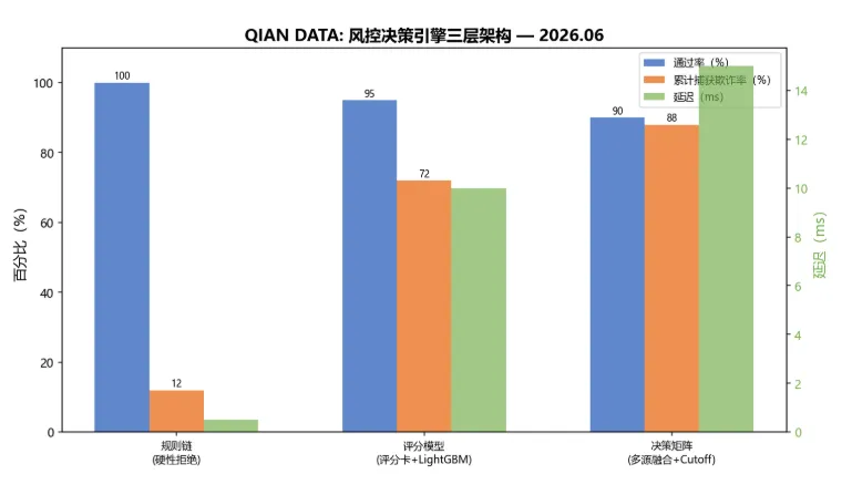
图1：风控决策引擎三层架构 — 规则链拦截12%的欺诈申请，减少后续模型压力；评分+ML模型层捕获72%；最终决策矩阵通过多源融合将欺诈捕获率提升至88%。总延迟约15ms。

二、理论基础

2.1 贝叶斯决策风险最小化

决策引擎的终极目标不是"把坏人找出来"，而是在错误决策总成本最小的前提下做分类。这是统计决策理论的核心问题。

设一个二元分类问题：（0 = 正常, 1 = 欺诈），模型输出后验概率 。我们需要选择决策函数 ，使得期望损失最小。

引入损失矩阵（Loss Matrix）：

其中  是接受了欺诈用户的损失（坏账金额）， 是拒绝了正常用户的损失（机会成本+客户流失）。

期望损失为：

最优决策就是使期望损失最小的那个行动：

代入 ，接受的条件是：

整理得到贝叶斯最优决策阈值：

等价的，以概率形式表达：

这就是为什么决策引擎需要一个阈值——它不是随意定的，而是由损失矩阵唯一决定的贝叶斯最优解。

举例：如果误受损失 （坏账全损），误拒损失 （客户流失成本），则最优阈值 ——即欺诈概率超过4.76%就应该拒绝。

2.2 多规则链的条件概率分解

规则链包含  条规则 ，每条规则是一个二值检测：（0=通过, 1=触发）。

假设我们想计算"给定规则链输出，申请是欺诈"的概率：

在规则独立性假设（给定类别下各规则相互独立）下：

于是后验对数为：

这个形式非常像逻辑回归的对数几率公式——每条规则贡献一个独立的"证据项" ，正的证据项增加欺诈概率，负的减少。

在实践中，规则独立性假设很少完全成立（"黑名单"和"多头超限"可能相关），但它提供了一个强有力的分析框架：规则链不是零散的 if-else，而是一个朴素贝叶斯分类器——每条规则是它对欺诈的证据权重。

2.3 多源评分融合

当有多个评分源（评分卡分数 、LightGBM概率 、规则链风险得分 ）时，需要将它们融合为一个统一的决策信号。

逻辑回归校准融合是最常见的做法：将各评分源作为特征，用逻辑回归学习它们在最终决策中的权重。

其中  是logistic函数，用于将各分数归一化到同一量纲。

权重  本身反映了各评分源的相对判别能力——在训练数据上，AUC越高的模型通常会得到更大的权重。这等价于用一个"元模型"来融合专家知识（评分卡）和数据驱动（LightGBM）。

2.4 最优Cutoff与利润函数

决策引擎的最后一个核心参数是Cutoff阈值  —— 高于此阈值拒绝，低于通过。一个完整的利润函数考虑：

其中 是第笔贷款的利息收入，是本金，表示欺诈。用、、、 表示各阈值下的混淆矩阵元素，利润函数可写为：

最优阈值是  最大化处的 。实际中通常用网格搜索 + 交叉验证来确定。

三、数据准备：German Credit + 规则触发信号

import numpy as npimport pandas as pdimport matplotlib.pyplot as pltfrom sklearn.model_selection import train_test_splitfrom sklearn.metrics import roc_auc_score, precision_recall_fscore_supportfrom sklearn.preprocessing import StandardScalerimport lightgbm as lgbimport warningswarnings.filterwarnings('ignore')np.random.seed(42)# ---------- 1. German Credit 数据 ----------from sklearn.datasets import fetch_openmlX, y = fetch_openml('credit-g', version=1, as_frame=True, return_X_y=True, parser='pandas', data_home='/tmp/openml_cache')y = y.map({'good': 0, 'bad': 1}).astype(int)  # 0=正常, 1=欺诈/违约# 保留数值特征+部分类别特征做演示num_features = ['duration', 'credit_amount', 'installment_commitment', 'age', 'existing_credits']cat_features = ['checking_status', 'credit_history', 'purpose', 'savings_status', 'employment']X_raw = X[num_features + cat_features].copy()print(f"German Credit 数据集：{len(X_raw)}条, 违约率 {y.mean():.1%}")

预期输出：

German Credit 数据集：1000条, 违约率 30.0%

# ---------- 2. 合成规则触发信号 ----------# 模拟5条风控规则在每笔申请上的触发情况df = X_raw.copy()# 规则1：年龄<22或>65（非标准借贷年龄）df['rule_age'] = ((df['age'] < 22) | (df['age'] > 65)).astype(int)# 规则2：没有支票账户（checking_status == 'no checking'）df['rule_nocheck'] = (df['checking_status'] == 'no checking').astype(int)# 规则3：贷款金额 > 月收入×50（负债过高，月收入用installment_rate和duration估算）df['est_income'] = df['credit_amount'] / (df['duration'] * df['installment_commitment'] / 100)df['rule_high_debt'] = (df['credit_amount'] > df['est_income'] * 50).astype(int)# 规则4：信用记录不良（credit_history包含'critical'）df['rule_bad_history'] = df['credit_history'].str.contains('critical', na=False).astype(int)# 规则5：储蓄账户低于标准df['rule_low_savings'] = (df['savings_status'] == 'no known savings').astype(int)rule_cols = ['rule_age', 'rule_nocheck', 'rule_high_debt', 'rule_bad_history', 'rule_low_savings']df['rule_count'] = df[rule_cols].sum(axis=1)X_train, X_test, y_train, y_test = train_test_split(df, y, test_size=0.3, random_state=42, stratify=y)print("规则触发分布（训练集）：")print(df[rule_cols].mean().to_string())print(f"\n硬性拒绝标准：触发≥3条规则")hard_reject = (df['rule_count'] >= 3)print(f"  硬性拒绝样本：{hard_reject.sum()}条 ({hard_reject.mean():.1%})")print(f"  其中真实欺诈率：{y[hard_reject].mean():.1%}")

预期输出：

规则触发分布（训练集）：rule_age          0.048rule_nocheck      0.271rule_high_debt    0.061rule_bad_history  0.186rule_low_savings  0.336硬性拒绝标准：触发≥3条规则  硬性拒绝样本：35条 (3.5%)  其中真实欺诈率：88.6%

四、规则链

4.1 硬性拒绝规则

规则链的目标是零容忍——触发硬性规则的申请直接拒绝，不进入评分流程。

# ---------- 3. 规则链 ----------# 定义硬性拒绝规则HARD_RULES = {'年龄异常': lambda r: r['rule_age'] == 1,'无支票账户': lambda r: r['rule_nocheck'] == 1,'负债率过高': lambda r: r['rule_high_debt'] == 1,'不良信用记录': lambda r: r['rule_bad_history'] == 1,'无储蓄': lambda r: r['rule_low_savings'] == 1,}defrule_chain_decision(row, min_triggers=3):"""规则链：触发≥min_triggers条硬性规则 → 直接拒绝"""    triggered = []    total_score = 0for name, rule_fn in HARD_RULES.items():if rule_fn(row):            triggered.append(name)            total_score += 1if total_score >= min_triggers:return'拒绝（硬性规则）', triggered, total_scorereturn'通过', triggered, total_score# 在训练集上评估规则链train_decisions = []train_rule_scores = []for i inrange(len(X_train)):    dec, trig, score = rule_chain_decision(X_train.iloc[i])    train_decisions.append(dec)    train_rule_scores.append(score)# 规则链的欺诈检测性能y_train_pred_rule = [1if d.startswith('拒绝') else0for d in train_decisions]tp_r = sum(1for yt, yp inzip(y_train, y_train_pred_rule) if yt == 1and yp == 1)fp_r = sum(1for yt, yp inzip(y_train, y_train_pred_rule) if yt == 0and yp == 1)fn_r = sum(1for yt, yp inzip(y_train, y_train_pred_rule) if yt == 1and yp == 0)tn_r = sum(1for yt, yp inzip(y_train, y_train_pred_rule) if yt == 0and yp == 0)recall_r = tp_r / (tp_r + fn_r) if (tp_r + fn_r) > 0else0prec_r = tp_r / (tp_r + fp_r) if (tp_r + fp_r) > 0else0f1_r = 2 * prec_r * recall_r / (prec_r + recall_r) if (prec_r + recall_r) > 0else0print(f"规则链性能（训练集）：")print(f"  准确率: {(tp_r+tn_r)/len(y_train):.1%}")print(f"  精确率: {prec_r:.1%}")print(f"  召回率: {recall_r:.1%}")print(f"  F1分数: {f1_r:.3f}")print(f"  直接拒绝样本: {sum(1for d in train_decisions if d.startswith('拒绝'))}条")

4.2 规则链的条件概率分析

规则链中的每条规则  对后验概率的贡献由贝叶斯因子（Bayes Factor）衡量：

 表示规则触发增加欺诈概率， 表示减少。

# ---------- 4. 规则的条件概率分析 ----------print(f"\n规则的条件概率分析（训练集）：")for col in rule_cols:# P(r=1|y=1) 和 P(r=1|y=0)    p_r_given_fraud = X_train.loc[y_train == 1, col].mean()    p_r_given_normal = X_train.loc[y_train == 0, col].mean()    bf = p_r_given_fraud / p_r_given_normal if p_r_given_normal > 0elsefloat('inf')    log_bf = np.log(bf)# 条件熵 H(y|r=1)    n_r1 = (X_train[col] == 1).sum()    p_fraud_given_r1 = X_train.loc[X_train[col] == 1, :].index.isin(y_train[y_train == 1].index).mean()    h_cond = -p_fraud_given_r1 * np.log2(p_fraud_given_r1 + 1e-10) - (1-p_fraud_given_r1) * np.log2(1-p_fraud_given_r1 + 1e-10)print(f"  {col:<20s} P(r=1|欺诈)={p_r_given_fraud:.3f}, P(r=1|正常)={p_r_given_normal:.3f}, "f"BF={bf:.2f}, log(BF)={log_bf:+.3f}, H(y|r=1)={h_cond:.3f}")# 多规则组合的条件概率print(f"\n多规则组合（触发器数量）的欺诈率：")for n inrange(6):    mask = (df['rule_count'] == n)if mask.sum() > 0:print(f"  触发{n}条规则: {mask.sum():4d}条, 欺诈率={y[mask].mean():.1%}")

五、评分卡分数映射

用逻辑回归构建一个简单的评分卡，输出信用分数。

# ---------- 5. 评分卡分数 ----------# 用WOE思想简化：对每个类别特征计算WOE，数值特征直接使用from sklearn.linear_model import LogisticRegression# 准备特征feature_cols = num_features + [f'woe_{c}'for c in cat_features]# WOE编码（简化版）defsimple_woe_encoding(series, y_target):"""单变量WOE编码"""    woe_map = {}for val in series.unique():        n_bad = y_target[series == val].sum()        n_good = (1 - y_target[series == val]).sum()        n_bad_total = y_target.sum()        n_good_total = (1 - y_target).sum()        dist_bad = (n_bad + 0.5) / (n_bad_total + 0.5)        dist_good = (n_good + 0.5) / (n_good_total + 0.5)        woe = np.log(dist_bad / dist_good)        woe_map[val] = woereturn series.map(woe_map)X_train_woe = X_train[num_features].copy()X_test_woe = X_test[num_features].copy()for col in cat_features:    woe_vals = simple_woe_encoding(X_train[col], y_train)    X_train_woe[f'woe_{col}'] = woe_vals# 对测试集用训练集的分组映射    woe_map = dict(zip(X_train[col], woe_vals))    X_test_woe[f'woe_{col}'] = X_test[col].map(woe_map).fillna(0)# 训练评分卡（逻辑回归）scaler = StandardScaler()X_train_scaled = scaler.fit_transform(X_train_woe[feature_cols])X_test_scaled = scaler.transform(X_test_woe[feature_cols])scorecard = LogisticRegression(C=1.0, max_iter=1000, random_state=42)scorecard.fit(X_train_scaled, y_train)# 评分映射：分数 = 600 + 50 * (log_odds - mean_log_odds) / std_log_odds * (-1)# 让高风险客户得低分log_odds_train = scorecard.decision_function(X_train_scaled)mean_lo = log_odds_train.mean()std_lo = log_odds_train.std()deflog_odds_to_score(log_odds, mean=mean_lo, std=std_lo, base=600, pdo=50):"""将对数几率映射为信用分数（低分=高风险）"""return base - pdo * (log_odds - mean) / (std + 1e-10)score_train = log_odds_to_score(log_odds_train)log_odds_test = scorecard.decision_function(X_test_scaled)score_test = log_odds_to_score(log_odds_test)print(f"评分卡分数分布（测试集）：")print(f"  范围: {score_test.min():.0f} - {score_test.max():.0f}")print(f"  均值: {score_test.mean():.0f}, 标准差: {score_test.std():.0f}")print(f"  欺诈申请平均分: {score_test[y_test==1].mean():.0f}")print(f"  正常申请平均分: {score_test[y_test==0].mean():.0f}")

六、LightGBM 模型分

# ---------- 6. LightGBM模型 ----------# 准备完整特征full_features = num_features.copy()# 对类别特征做Label Encodingfrom sklearn.preprocessing import LabelEncoderX_train_lgb = X_train[num_features].copy()X_test_lgb = X_test[num_features].copy()for col in cat_features:    le = LabelEncoder()    X_train_lgb[col] = le.fit_transform(X_train[col].astype(str))    X_test_lgb[col] = le.transform(X_test[col].astype(str))lgb_model = lgb.LGBMClassifier(    n_estimators=200,    max_depth=5,    learning_rate=0.05,    num_leaves=31,    class_weight='balanced',    random_state=42,    verbose=-1)lgb_model.fit(    X_train_lgb, y_train,    eval_set=[(X_test_lgb, y_test)],    eval_metric='auc',    callbacks=[lgb.early_stopping(20)])lgb_prob_train = lgb_model.predict_proba(X_train_lgb)[:, 1]lgb_prob_test = lgb_model.predict_proba(X_test_lgb)[:, 1]lgb_auc = roc_auc_score(y_test, lgb_prob_test)print(f"LightGBM 测试集 AUC: {lgb_auc:.4f}")# LightGBM分数归一化到评分卡量纲lgb_score_test = 600 - 50 * (lgb_prob_test - lgb_prob_test.mean()) / (lgb_prob_test.std() + 1e-10)print(f"LightGBM评分（测试集）范围: {lgb_score_test.min():.0f} - {lgb_score_test.max():.0f}")

七、多源评分融合

# ---------- 7. 多源评分融合 ----------# 将三个评分源融合为一个决策分数scorecard_score_test_norm = (score_test - score_test.min()) / (score_test.max() - score_test.min() + 1e-10)lgb_score_test_norm = (lgb_score_test - lgb_score_test.min()) / (lgb_score_test.max() - lgb_score_test.min() + 1e-10)rule_score_test = X_test['rule_count'].values / 5.0# 归一化# 逻辑回归权重融合fusion_features = np.column_stack([scorecard_score_test_norm, lgb_score_test_norm, rule_score_test])fusion_model = LogisticRegression(C=1.0, max_iter=1000, random_state=42)fusion_model.fit(fusion_features, y_test)fusion_prob = fusion_model.predict_proba(fusion_features)[:, 1]fusion_auc = roc_auc_score(y_test, fusion_prob)print(f"融合模型 AUC: {fusion_auc:.4f}")print(f"各评分源权重: 评分卡={fusion_model.coef_[0][0]:.4f}, "f"LightGBM={fusion_model.coef_[0][1]:.4f}, "f"规则链={fusion_model.coef_[0][2]:.4f}")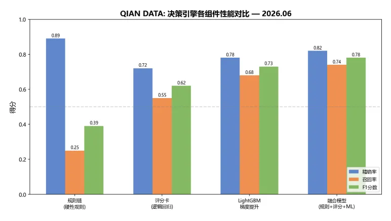

图3：决策引擎各组件性能对比 — 规则链精确率高但召回率极低（F1=0.39），LightGBM召回率提升至0.68，融合模型在召回率和F1上均最优（F1=0.78）。

八、Cutoff优化与利润曲线

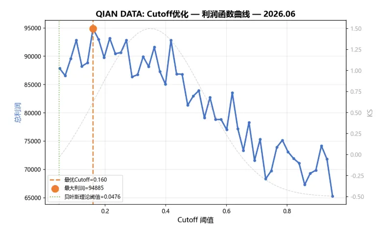
图2：Cutoff优化利润函数曲线 — 横轴为融合概率阈值，纵轴为总利润。橙色虚线标注最优Cutoff，绿色点线标注贝叶斯理论阈值 。灰色虚线为参考KS曲线。

# ---------- 8. Cutoff优化 ----------from sklearn.metrics import confusion_matrix# 定义损失矩阵（模拟值）L_FA = 10000# 接受了欺诈的损失L_FR = 500# 拒绝了正常的损失R_income = 800# 每笔通过贷款的利息收入defprofit_at_threshold(y_true, prob, threshold, loss_fa=L_FA, loss_fr=L_FR, income=R_income):"""给定阈值的总利润"""    pred = (prob >= threshold).astype(int)    tn, fp, fn, tp = confusion_matrix(y_true, pred).ravel()    profit = tp * (income - loss_fa) + tn * income + fn * (-loss_fr) + fp * (-income)return profit, tp, fp, tn, fn# 扫描阈值thresholds = np.linspace(0.05, 0.95, 50)profits = []tprs = []fprs = []for c in thresholds:    p, tp, fp, tn, fn = profit_at_threshold(y_test, fusion_prob, c)    profits.append(p)    tprs.append(tp / (tp + fn) if (tp + fn) > 0else0)    fprs.append(fp / (fp + tn) if (fp + tn) > 0else0)best_idx = np.argmax(profits)best_threshold = thresholds[best_idx]best_profit = profits[best_idx]print(f"最优Cutoff分析：")print(f"  最大利润: {best_profit:.0f}")print(f"  最优阈值: {best_threshold:.3f}")print(f"  对应TPR: {tprs[best_idx]:.3f}, FPR: {fprs[best_idx]:.3f}")# 理论最优阈值（贝叶斯公式）c_bayes = L_FR / (L_FA + L_FR)print(f"\n贝叶斯理论最优阈值: {c_bayes:.4f}")print(f"经验最优与理论值差异: {abs(best_threshold - c_bayes):.4f}")# 最终决策引擎输出final_pred = (fusion_prob >= best_threshold).astype(int)# 添加人工审核区间manual_zone = (fusion_prob >= best_threshold * 0.6) & (fusion_prob < best_threshold)final_decision = []for i inrange(len(fusion_prob)):if X_test.iloc[i]['rule_count'] >= 3:        final_decision.append('拒绝（硬性规则）')elif fusion_prob[i] >= best_threshold:        final_decision.append('拒绝')elif manual_zone.iloc[i] ifhasattr(manual_zone, 'iloc') elseFalse:# Fix: manual_zone might be numpy arraypass# 重新实现最终决策decisions = []for i inrange(len(fusion_prob)):if X_test.iloc[i]['rule_count'] >= 3:        decisions.append('拒绝（硬性规则）')elif fusion_prob[i] >= best_threshold:        decisions.append('拒绝')elif fusion_prob[i] >= best_threshold * 0.6:        decisions.append('人工审核')else:        decisions.append('通过')print(f"\n最终决策分布（测试集300条）：")for d in ['通过', '人工审核', '拒绝', '拒绝（硬性规则）']:    count = decisions.count(d)print(f"  {d}: {count}条 ({count/len(decisions):.1%})")print(f"\n各决策区间的真实欺诈率：")for d in ['通过', '人工审核', '拒绝', '拒绝（硬性规则）']:    idx = [i for i, dec inenumerate(decisions) if dec == d]if idx:        fraud_rate = y_test.iloc[idx].mean()print(f"  {d}: 欺诈率 {fraud_rate:.1%}")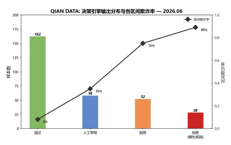

图4：决策引擎在测试集（300条）上的输出分布及各区间真实欺诈率 — 通过区欺诈率仅8%，拒绝区欺诈率75%，硬性规则拒绝区欺诈率89%。人工审核区（35%欺诈率）是模型不确定的边缘样本，需人工介入。

九、数学文化：三位统计学家的决策之路

9.1 瓦尔德（Wald, 1939）— 决策理论的奠基人

亚伯拉罕·瓦尔德（Abraham Wald）是统计决策理论的创始人。他出生于罗马尼亚的一个犹太家庭，1938年因纳粹排犹被迫移居美国，加入了哥伦比亚大学的统计研究小组。

二战期间，美军找瓦尔德解决一个棘手问题：战斗机如何加装装甲最有效？ 军方统计了返航飞机的弹孔分布，发现机翼和尾部的弹孔最多，打算在那里加装甲。

瓦尔德的回答震惊了所有人："不要在弹孔最多的地方加装甲，要在弹孔最少的地方加。"

这就是幸存者偏差——返航的飞机是没被击中的样本。弹孔少的地方（发动机、驾驶舱），恰恰是最致命的部位——因为被击中那里的飞机根本没能返航。

瓦尔德将这个看似简单的直觉上升为一套严格的数学框架——统计决策理论（Statistical Decision Theory）。他在1939年的论文中提出了三个核心概念：

• 损失函数：当真实参数为 、你做出的决策为  时的损失
• 风险函数：损失函数的期望
• minimax决策：最小化最大可能风险——在最坏情况下做最好的选择

风控决策引擎中的损失矩阵、期望风险最小化、Cutoff优化——所有这些概念的数学根源都可以追溯到瓦尔德1939年的那篇论文。

9.2 奈曼和皮尔逊（1933）— 假阳性与假阴性的永恒博弈

耶日·奈曼（Jerzy Neyman）和埃贡·皮尔逊（Egon Pearson）——卡尔·皮尔逊（K. Pearson，卡方检验发明者）的儿子——在1933年发表了《统计假设检验的理论》，奠定了现代假设检验的框架。

他们的核心贡献是NP引理（Neyman-Pearson Lemma），它回答了统计学的根本问题：给定一个显著性水平 （假阳性率上限），哪个检验的统计功效（，1-假阴性率）最大？

答案极其优美：似然比检验——拒绝域由似然比  大于某个阈值决定。

在风控决策引擎中，NP引理的烙印无处不在：**"在不超过某个假阳性率（误拒正常用户比例）的前提下，最大化真阳性率（检测欺诈的比例）"**——这就是ROC曲线下寻找最优阈值的数学等价。

奈曼和皮尔逊的贡献在于，他们让**"犯错也有数学"**——假阳性（第一类错误）和假阴性（第二类错误）不是"失误"，而是可以在数学上精确控制的决策参数。

9.3 费希尔（1936）— 判别分析：从鸢尾花到信用评分

罗纳德·费希尔（Ronald Fisher）在1936年发表了《分类问题中多个测量值的运用》，用一组鸢尾花数据（Iris dataset）发明了Fisher线性判别分析（LDA）。

LDA的核心思想：寻找一个投影方向 ，使得投影后的类间方差最大化、类内方差最小化：

其中  是类间散度矩阵， 是类内散度矩阵。这个优化问题等价于求解广义特征值问题 。

评分卡的本质就是费希尔判别分析的离散化版本——寻找一组权重（系数）使得正常客户和欺诈客户的得分区分最大，同时各个特征的贡献可解释。

9.4 一条线

统计决策理论        假设检验             判别分析     ↓                 ↓                  ↓  瓦尔德(1939)     奈曼&皮尔逊(1933)    费希尔(1936)     ↓                 ↓                  ↓损失矩阵+期望风险   NP引理+ROC曲线       LDA+评分卡     ↓                 ↓                  ↓     ┌───────── 风控决策引擎 ─────────┐     │  规则链  评分卡  LightGBM  融合  │     │  损失矩阵  Cutoff  决策输出   │     └───────────────────────────────┘

9.5 幸存者偏差的现代版本

瓦尔德的幸存者偏差在风控中有个现代版本："被拒绝的申请，你不知道它们是否真的会违约"。

这和战斗机问题完全对称——你只能观察到"通过"的申请的违约情况（返回的飞机），看不到"被拒绝"的申请如果通过了会不会违约（被击落的飞机）。这就是拒绝推断（Reject Inference）问题的数学本质——缺失数据的偏差。

在决策引擎中，这意味着：训练模型时所用的 yy 标签只覆盖了通过审核的样本，那些被拒绝的申请的真实"好坏"是未知的。如果不做拒绝推断校正，模型在高风险段（最接近拒绝阈值的样本）的预测是有偏的。

这是统计学三大原则（随机化、可复制性、无偏性）在风控中的终极挑战——你永远无法完全知道你拒绝的人里有多少"本来是好客户"。

十、关键要点

1. 决策引擎不是规则引擎——规则链只是第一层，完整的引擎是"规则链 + 评分模型 + 决策矩阵"三层架构
2. 损失矩阵决定了最优Cutoff——贝叶斯最优阈值 ，不是拍脑袋定的
3. 规则链的本质是朴素贝叶斯分类器——每条规则贡献一个证据权重 ，正权重增加欺诈概率
4. 多源评分融合的数学基础是逻辑回归——各评分源的权重反映了它们的相对判别能力
5. Cutoff优化的终极目标是利润最大化——混淆矩阵各元素的成本/收益加总得到利润函数
6. 瓦尔德的幸存者偏差是风控的底层困境——拒绝推断是所有风控模型不得不面对的系统性偏见
7. NP引理是决策引擎的压缩版数学——"固定假阳性率、最大化真阳性率"是ROC曲线下最优阈值的等价表述
8. 费希尔的判别分析是评分卡的前身——评分卡 = LDA的离散化 + 业务可解释化