Python绘图 | Nature桑基图复现(包含完整代码)
- 2026-06-30 20:23:20
Python绘图 | Nature桑基图复现(包含完整代码)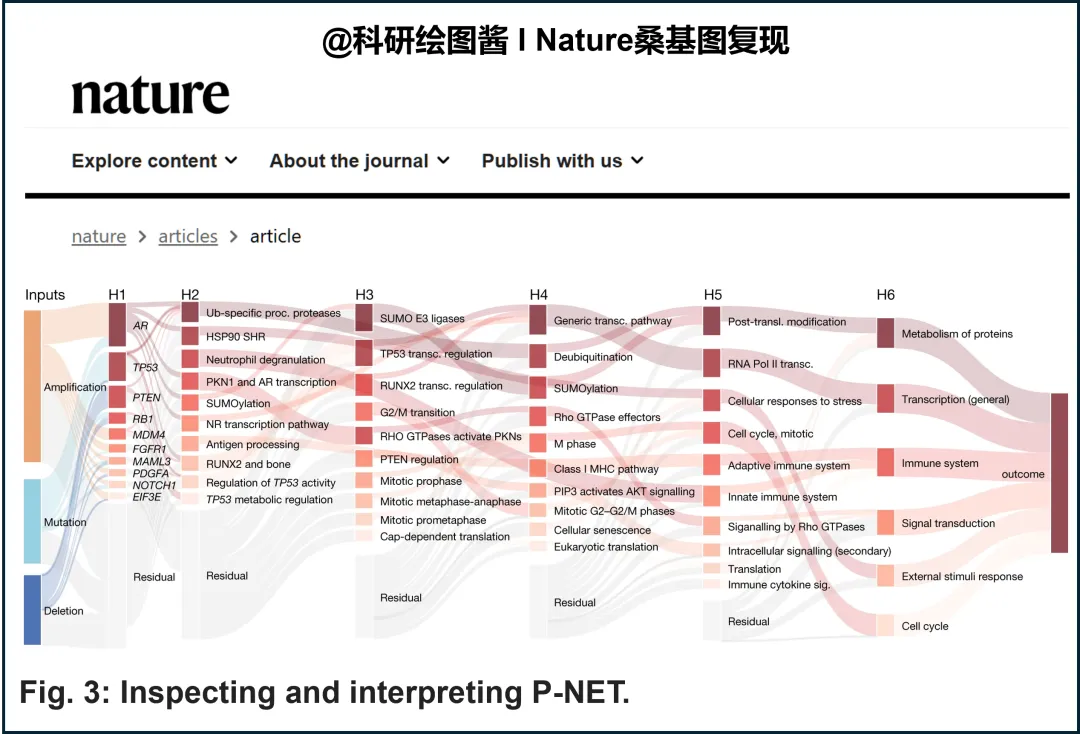
复现前后对比: 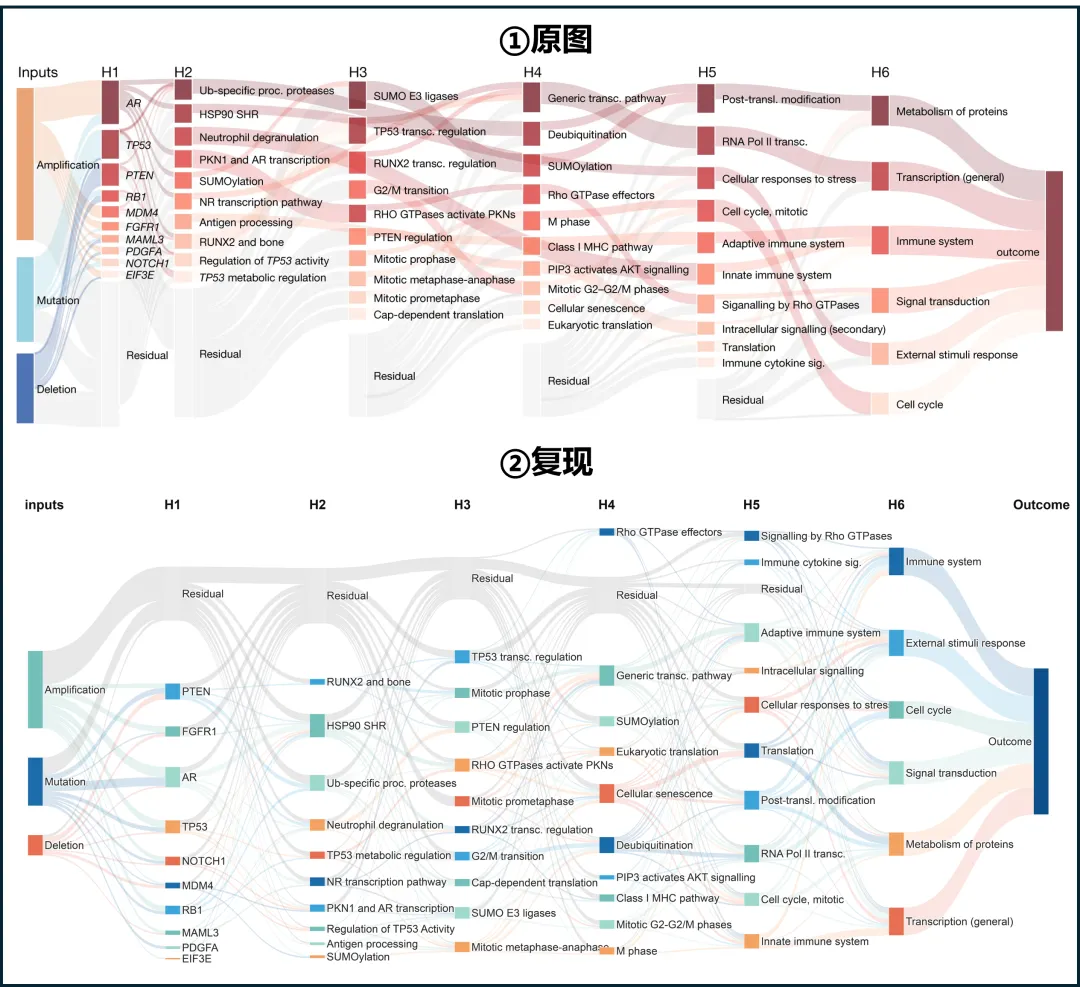
下面展示了如何用Python复现的过程(数据为模拟据);我们根据三大主流顶刊Cell, Nature和Science的配色风格设置了不同的绘图类型。 1. 绘图代码(此处所用到的sankey是我们开发的软件包): 2. 绘图主代码(自主开发的sankey): ①Nature配色风格: 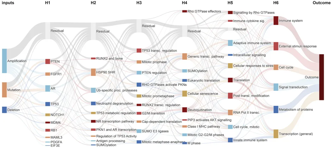
②Cell配色风格: 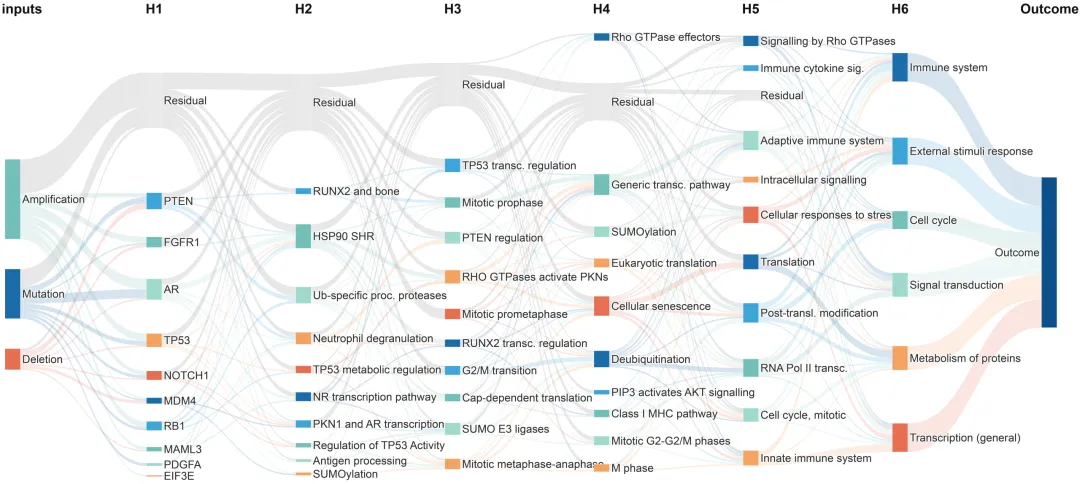
③Science配色风格: 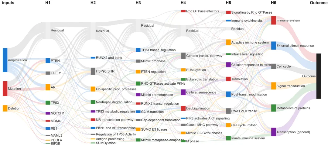
好了,本期内容到此结束,喜欢的小伙伴可以转发分享,收藏,别忘了来个三连击啊~~~ 【制作不易,获取请扫码获取或者点击链接】 https://mbd.pub/o/author-bWeVnG5law== 
Python绘图 | 复现顶刊中机器学习SHAP特征重要性交互网络与个性化解释图(包含完整代码) R绘图 | Science网络相关性热图复现(包含完整代码) R绘图 | NC相关性矩阵热图复现(包含完整代码) R绘图 | CNS 级相关性矩阵热图复现进阶教程(含完整代码) Python绘图 | Nature不同细胞类型中标记基因的表达点图复现(包含完整代码) R绘图 | Nature山脊图复现(包含完整代码) R绘图 | Nature散点配对连线图(包含完整代码) Python绘图 | NC变量相关性散点图复现(包含完整代码) R绘图 | NC主成分PCA图复现(包含完整代码)

添加小编微信进群交流学习!
桑基图(Sankey Diagram),多层样式常称冲积图,核心用于流向与层级关系可视化。图表由节点、流线两大基础元素构成,遵循从左到右的阅读逻辑,流线宽度直观反映数据权重、数量或占比。其优势在于同时呈现传递路径、类别关联与规模差异,适合分析多分支、多阶段的连续流程。在科研场景中,多用于解析基因变异、信号通路、代谢过程与疾病表型的传导关系;应用领域包括但不限于农学、生态学,可展示种质分类、物质循环、种群及环境因子的流转规律;也普遍用于各类实验分组、分子组学数据、化学反应流程等链式数据分析,是呈现科研复杂流程与关联关系的常用图表。原图源于Nature 顶刊上的一篇文献:Biologically informed deep neural network for prostate cancer discovery。下面展示了Python绘制这类图的全部过程,供大家参考。
原文中的结果图:Fig. 3
Python代码
import os, numpy as np, pandas as pdfrom sankey import sankeyos.makedirs("./result/paper_figures", exist_ok=True)# ═══════════════════════════════════════════════════════════# 1. Node definitions# ═══════════════════════════════════════════════════════════INPUTS = ["Amplification", "Mutation", "Deletion"]H1 = ["AR", "TP53", "PTEN", "RB1", "MDM4","FGFR1", "MAML3", "PDGFA", "NOTCH1", "EIF3E", "Residual"]H2 = ["Ub-specific proc. proteases", "HSP90 SHR","Neutrophil degranulation", "PKN1 and AR transcription","SUMOylation", "NR transcription pathway","Antigen processing", "RUNX2 and bone","Regulation of TP53 Activity", "TP53 metabolic regulation","Residual"]H3 = ["SUMO E3 ligases", "TP53 transc. regulation","RUNX2 transc. regulation", "G2/M transition","RHO GTPases activate PKNs", "PTEN regulation","Mitotic prophase", "Mitotic metaphase-anaphase","Mitotic prometaphase", "Cap-dependent translation","Residual"]H4 = ["Generic transc. pathway", "Deubiquitination","SUMOylation", "Rho GTPase effectors","M phase", "Class I MHC pathway","PIP3 activates AKT signalling", "Mitotic G2-G2/M phases","Cellular senescence", "Eukaryotic translation","Residual"]H5 = ["Post-transl. modification", "RNA Pol II transc.","Cellular responses to stress", "Cell cycle, mitotic","Adaptive immune system", "Innate immune system","Signalling by Rho GTPases", "Intracellular signalling","Translation", "Immune cytokine sig.","Residual"]H6 = ["Metabolism of proteins", "Transcription (general)","Immune system", "Signal transduction","External stimuli response", "Cell cycle"]OUTCOME = ["Outcome"]# ═══════════════════════════════════════════════════════════# 2. Sampling probabilities# ═══════════════════════════════════════════════════════════PROBS = {"Inputs": [0.50, 0.30, 0.20],"H1": [0.14, 0.09, 0.08, 0.07, 0.06, 0.05, 0.04, 0.03, 0.02, 0.02, 0.38],"H2": [0.10, 0.08, 0.08, 0.06, 0.06, 0.06, 0.04, 0.04, 0.04, 0.04, 0.40],"H3": [0.12, 0.09, 0.08, 0.07, 0.06, 0.06, 0.06, 0.06, 0.06, 0.06, 0.28],"H4": [0.12, 0.09, 0.08, 0.07, 0.06, 0.06, 0.06, 0.06, 0.06, 0.06, 0.28],"H5": [0.12, 0.14, 0.10, 0.10, 0.10, 0.10, 0.10, 0.05, 0.05, 0.06, 0.08],"H6": [0.20, 0.20, 0.20, 0.15, 0.15, 0.10],"Outcome": [0.5],}ALL_NODES = {"Inputs": INPUTS,"H1": H1,"H2": H2,"H3": H3,"H4": H4,"H5": H5,"H6": H6,"Outcome": OUTCOME,}# ═══════════════════════════════════════════════════════════# 3. Simulate data# ═══════════════════════════════════════════════════════════def simulate_r_style(n: int = 100, seed: int = 42) -> pd.DataFrame:rng = np.random.default_rng(seed)data = {}for layer in ["Inputs", "H1", "H2", "H3", "H4", "H5", "H6", "Outcome"]:nodes = ALL_NODES[layer]probs = np.array(PROBS[layer])probs = probs / probs.sum()data[layer] = rng.choice(nodes, size=n, p=probs)return pd.DataFrame(data)df = simulate_r_style(n=100, seed=42)print(f"Simulated: {len(df)} rows x {len(df.columns)} columns")for col in df.columns:counts = df[col].value_counts()print(f" {col}: {dict(counts)}")
# ═══════════════════════════════════════════════════════════# 4. 自主开发的sankey绘图包# ═══════════════════════════════════════════════════════════nature_custom = {"main_palette": ["#7B1515", "#B54848", "#D4956A", "#8BBDD4", "#4A6FAF", "#C4A35A"],"gradient_method": "sequential","gradient_lighten": 0.6,"input_colors": ["#D4956A", "#8BBDD4", "#4A6FAF"],"residual_color": "#F0F0F0","residual_link_alpha": 0.38,"outcome_color": "#5A1010","outcome_link_alpha": 0.35,"default_link_alpha": 0.18,"font_family": "Arial","font_size": 18,"node_thickness": 25,"node_pad": 80,}layer_cols = ["Inputs", "H1", "H2", "H3", "H4", "H5", "H6", "Outcome"]## 我们开发的软件包最核心的一个函数 ###fig = sankey(df,layer_cols=layer_cols,preset=nature_custom,y_method="fixed_gap",gap=0.012,height=750,width=2200,)##################################### 输出路径base_path = "./result/paper_figures/sankey_nature"out_html = f"{base_path}.html"out_png = f"{base_path}.png"out_pdf = f"{base_path}.pdf"# 1. 保存交互式 HTMLfig.write_html(out_html)print(f"\nSaved HTML: {out_html}")# 2. 保存 PNG(scale 提高分辨率,论文推荐 scale=2~3)fig.write_image(out_png, width=1800, height=800, scale=2)print(f"Saved PNG: {out_png}")# 3. 保存 PDF(矢量图,期刊/论文首选,无损缩放)fig.write_image(out_pdf, width=1800, height=800)print(f"Saved PDF: {out_pdf}")
复现图如下
往期回顾
参考文献:Elmarakeby, H.A., Hwang, J., Arafeh, R. et al. Biologically informed deep neural network for prostate cancer discovery. Nature 598, 348–352 (2021). https://doi.org/10.1038/s41586-021-03922-4
以上内容为原创,转载需声明出处。
🔥亲测有效,一键运行,助你快速上手!
🔥整理不易,欢迎点赞分享给更多小伙伴~
本文来自网友投稿或网络内容,如有侵犯您的权益请联系我们删除,联系邮箱:wyl860211@qq.com 。
随机文章
-
 10个月宝宝每天需要喝多少奶粉?
- 豆瓣评分8.6 《零基础入门学习Python》零基础小白必备 建议收藏
- 别再复制粘贴了!用这个Python库,PDF拆分、合并、加密一键搞定
- 【粉丝真实需求】外贸办公 Python 自动化・提单水印批量实战 2/6
- Linux 内核 eBPF 程序挂载点与执行分析
- 算力平权第四波:从 Linux 到 TurboQuant,独立开发者又拿到一把新钥匙
- Linux buff/cache内存占用飙升?90%运维踩坑:盲目清缓存正在慢慢拖垮服务器
- 为什么sudo要输密码?Linux权限机制原来是这么设计的
- Linux Tickless 机制解析:从周期时钟中断到动态时钟管理
- 【开源Git】无需写python,也能玩转浏览器爬虫自动化(windows/mac)
- 为什么Linux游戏等了二十年,最后是被一台游戏机救活的?
