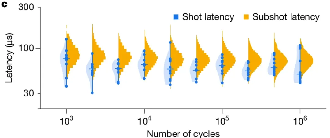
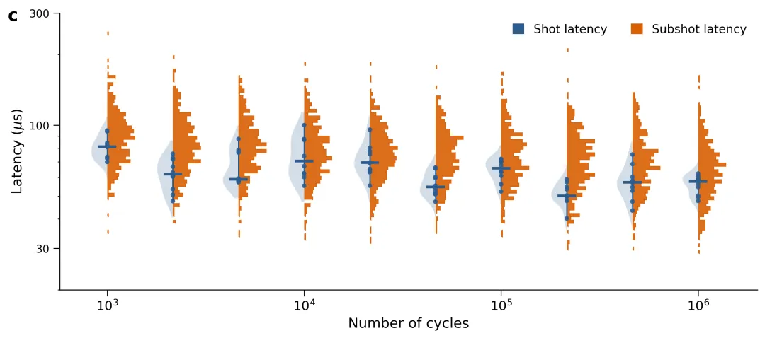
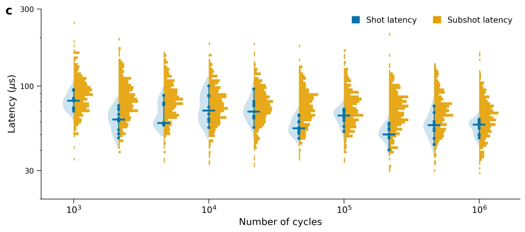
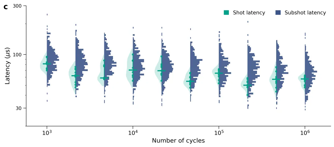
COLOR_PALETTES = { 1: {"shot": "#1E77F4", "subshot": "#F2A900"}, # Nature 风格标准科技蓝与高对比橙黄 2: {"shot": "#2B5C8F", "subshot": "#D95F02"}, # Science 常用经典深海蓝与明快朱红 3: {"shot": "#0072B2", "subshot": "#E69F00"}, # Cell 推荐色盲友好型高对比度深蓝与金黄 4: {"shot": "#00A087", "subshot": "#3C5488"}, # Lancet 柳叶刀经典薄荷绿与深邃海军蓝 5: {"shot": "#4DBBD5", "subshot": "#E64B35"}, # JAMA 美国医学会杂志现代天蓝与珊瑚红 6: {"shot": "#1170AA", "subshot": "#FC7D0B"}, # IEEE 电子学报标准科技深蓝与动感纯橙 7: {"shot": "#3F51B5", "subshot": "#FF5722"}, # Advanced Materials 先进材料高纯度靛蓝与亮橙 8: {"shot": "#1F77B4", "subshot": "#FF7F0E"}, # Matplotlib 经典标准学术蓝与活力橙 9: {"shot": "#4A6B82", "subshot": "#C87A53"}, # ACS 美国化学会常用低饱和度灰蓝与泥土赭 10: {"shot": "#3C4E5A", "subshot": "#E28743"}, # Royal Society 皇家学会工业质感冷灰蓝与暖铜 11: {"shot": "#2F4F4F", "subshot": "#D2691E"}, # Earth Science 地学期刊岩石深墨绿与质感巧克力棕 12: {"shot": "#4682B4", "subshot": "#F4A460"}, # Geophysical 研究简报渐变柔和钢蓝与沙滩浅黄 13: {"shot": "#008080", "subshot": "#CD853F"}, # Nature Climate Change 环保系青翠绿与沙漠金褐 14: {"shot": "#7B1FA2", "subshot": "#FFA000"}, # PRL 物理评论快报高能物理紫与高亮量子黄 15: {"shot": "#5C3D75", "subshot": "#E0B034"}, # Astronomy & Astrophysics 天体物理深邃星空紫与恒星金 16: {"shot": "#6A3D9A", "subshot": "#FF7F00"}, # BioMed Central 生物医学常用高纯紫与橙 17: {"shot": "#08519C", "subshot": "#A50F15"}, # PNAS 经典对比双色高饱和深蓝与高饱和深红 18: {"shot": "#238B45", "subshot": "#D94801"}, # Ecosystems 生态学植被深绿与土壤深橙 19: {"shot": "#54278F", "subshot": "#2171B5"}, # Grid Computing 分布式计算冷色调深紫与数字晶莹蓝 20: {"shot": "#2C3E50", "subshot": "#E74C3C"} # Wiley 材料学常用工业风石墨黑与醒目鲜红}
import osimport matplotlib.pyplot as pltimport numpy as npimport pandas as pdfrom scipy.stats import gaussian_kdefrom matplotlib.patches import Patch# 1. 自动创建图表文件夹output_dir = "图表"if not os.path.exists(output_dir): os.makedirs(output_dir)# 2. 从 Excel 中读取数据if not os.path.exists("data.xlsx"): raise FileNotFoundError("未找到 data.xlsx 文件,请先运行数据生成脚本。")df_shot = pd.read_excel("data.xlsx", sheet_name="Shot_Latency")df_subshot = pd.read_excel("data.xlsx", sheet_name="Subshot_Latency")# 获取所有的循环周期cycles = sorted(df_shot["Cycles"].unique())# 3. 符合主流期刊标准的专业科研配色方案COLOR_PALETTES = { 1: {"shot": "#1E77F4", "subshot": "#F2A900"}, # Nature 风格标准科技蓝与高对比橙黄}# 选择方案 1 作为绘图颜色selected_palette = COLOR_PALETTES[1]color_shot = selected_palette["shot"]color_subshot = selected_palette["subshot"]# 4. 初始化画布fig, ax = plt.subplots(figsize=(10, 4.5), dpi=300)# 5. 核心绘图逻辑for x_idx, cycle in enumerate(cycles): shot_vals = df_shot[df_shot["Cycles"] == cycle]["Latency"].values subshot_vals = df_subshot[df_subshot["Cycles"] == cycle]["Latency"].values x_pos = x_idx # --- 左侧:Shot Latency (半边小提琴) --- if len(shot_vals) > 0: shot_pts = shot_vals[:10] log_shot_pts = np.log10(shot_pts) kde = gaussian_kde(log_shot_pts) y_log_range = np.linspace(np.log10(20), np.log10(350), 300) kde_vals = kde(y_log_range) kde_vals = (kde_vals / kde_vals.max()) * 0.24 y_range = 10 ** y_log_range mask = (y_range >= shot_pts.min() * 0.85) & (y_range <= shot_pts.max() * 1.15) ax.fill_betweenx(y_range[mask], x_pos - kde_vals[mask], x_pos, color=color_shot, alpha=0.2, lw=0) ax.plot([x_pos, x_pos], [shot_pts.min(), shot_pts.max()], color=color_shot, lw=1.2, zorder=2) median_shot = np.median(shot_pts) ax.plot([x_pos - 0.12, x_pos + 0.12], [median_shot, median_shot], color=color_shot, lw=2.5, zorder=4) ax.scatter([x_pos] * len(shot_pts), shot_pts, color=color_shot, s=18, alpha=0.9, zorder=3, edgecolors='none') # --- 右侧:Subshot Latency (高密度精细直方图) --- if len(subshot_vals) > 0: log_subshot = np.log10(subshot_vals) counts, log_bins = np.histogram(log_subshot, bins=70, range=(np.log10(25), np.log10(250))) bins = 10 ** log_bins counts = (counts / counts.max()) * 0.42 for j in range(len(counts)): if counts[j] > 0: ax.fill_betweenx([bins[j], bins[j + 1]], x_pos, x_pos + counts[j], color=color_subshot, alpha=0.9, edgecolor=None, lw=0) ax.plot([x_pos + counts[j], x_pos + counts[j]], [bins[j], bins[j + 1]], color=color_subshot, lw=0.6) if j < len(counts) - 1 and counts[j + 1] > 0: ax.plot([x_pos + counts[j], x_pos + counts[j + 1]], [bins[j + 1], bins[j + 1]], color=color_subshot, lw=0.6)# 6. 坐标轴与图表美化ax.set_yscale('log')ax.set_ylim(20, 300)ax.set_yticks([30, 100, 300])ax.set_yticklabels(['30', '100', '300'])ax.get_yaxis().set_major_formatter(plt.ScalarFormatter())ax.set_ylabel(r'Latency ($\mu$s)', fontsize=13)target_indices = [idx for idx, c in enumerate(cycles) if np.log10(c).is_integer()]target_labels = [f"$10^{int(np.log10(cycles[idx]))}$" for idx in target_indices]ax.set_xticks(target_indices)ax.set_xticklabels(target_labels, fontsize=12)ax.set_xlabel('Number of cycles', fontsize=13)ax.spines['top'].set_visible(False)ax.spines['right'].set_visible(False)ax.spines['left'].set_linewidth(0.8)ax.spines['bottom'].set_linewidth(0.8)ax.tick_params(direction='out', length=6, width=0.8)legend_elements = [ Patch(facecolor=color_shot, label='Shot latency'), Patch(facecolor=color_subshot, label='Subshot latency')]ax.legend(handles=legend_elements, loc='upper right', frameon=False, ncol=2, fontsize=11, handlelength=1, handleheight=1)ax.text(-0.06, 1.02, 'c', transform=ax.transAxes, fontsize=16, fontweight='bold', va='top', ha='right')plt.tight_layout()# 7. 保存高清图表output_path = os.path.join(output_dir, "latency_chart.png")plt.savefig(output_path, bbox_inches='tight')plt.close()print(f"绘制完成,应用配色方案: {output_path}")