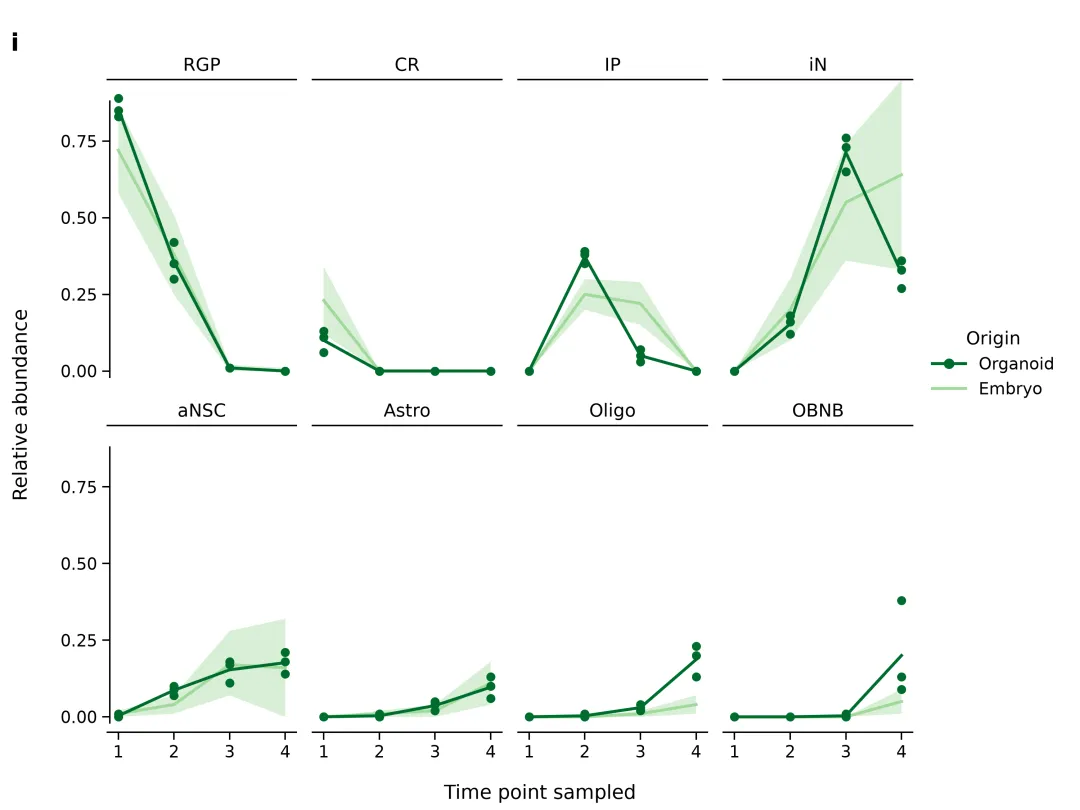
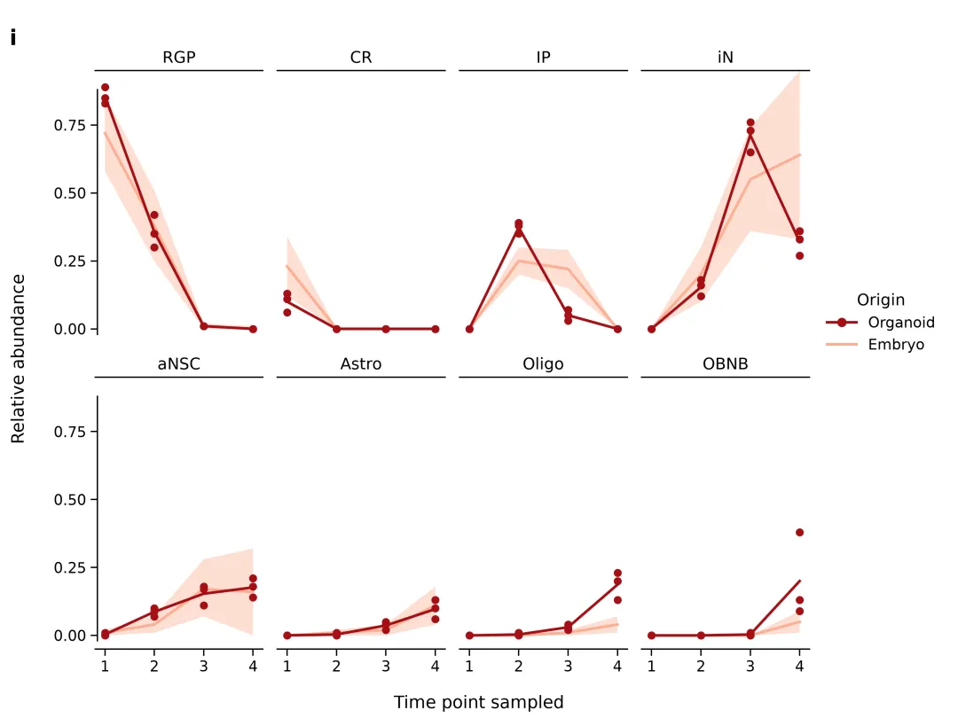
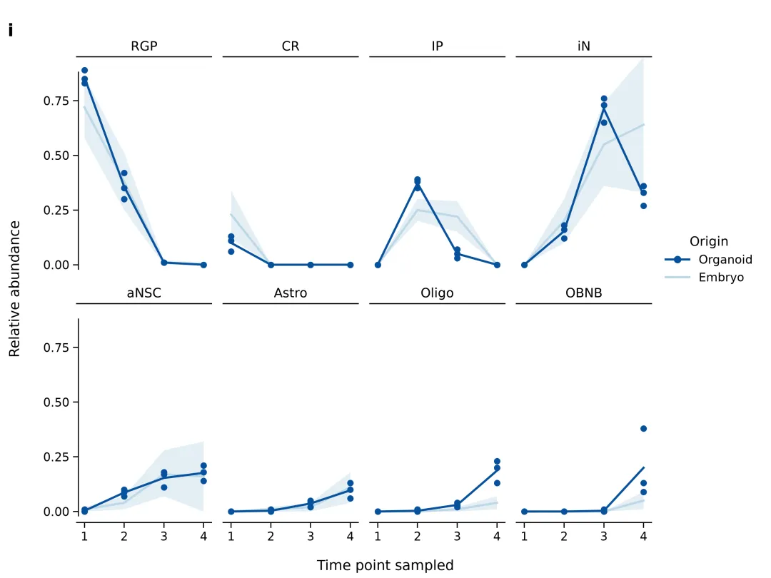
COLOR_PALETTES = {    1: {        "organoid": "#000000","embryo": "#7F7F7F",    },  # 经典黑灰 (Nature/Science单色常用风格)    2: {        "organoid": "#08519C", "embryo": "#BDD7E7",    },  # 经典蓝阶 (Cell/Lancet单色调水蓝)    3: {        "organoid": "#006D2C","embryo": "#A1D99B",    },  # 经典绿阶 (生物/生态学绿系对比)    4: {        "organoid": "#A50F15","embryo": "#FCAE91",    },  # 经典红阶 (医学/病理学暖红对比)    5: {        "organoid": "#542788","embryo": "#BCBDDC",    },  # 紫色调系 (分子生物/基因组学常用)    6: {        "organoid": "#E41A1C","embryo": "#377EB8",    },  # Red-Blue (经典Nature双色高对比)    7: {        "organoid": "#1B9E77","embryo": "#D95F02",    },  # Dark2-Green-Orange (PNAS/Cell经典高对比)    8: {        "organoid": "#4DAF4A","embryo": "#984EA3",    },  # Green-Purple (互补色高辨识度方案)    9: {        "organoid": "#377EB8","embryo": "#FF7F00",    },  # Blue-Orange (神经科学/冷暖对比)    10: {        "organoid": "#008080","embryo": "#E6AB02",    },  # Teal-Gold (Nature Medicine风格)    11: {        "organoid": "#1F77B4","embryo": "#AEC7E8",    },  # Tableau Blue (数据可视化标准深浅蓝)    12: {        "organoid": "#FF7F0E","embryo": "#FFBB78",    },  # Tableau Orange (数据可视化标准深浅橙)    13: {        "organoid": "#2CA02C","embryo": "#98DF8A",    },  # Tableau Green (数据可视化标准深浅绿)    14: {        "organoid": "#D62728","embryo": "#FF9896",    },  # Tableau Red (数据可视化标准深浅红)    15: {        "organoid": "#9467BD","embryo": "#C5B0D5",    },  # Tableau Purple (数据可视化标准深浅紫)    16: {        "organoid": "#8C564B","embryo": "#C49C94",    },  # Tableau Brown (沉稳大地色双阶)    17: {        "organoid": "#E377C2","embryo": "#F7B6D2",    },  # Tableau Pink (柔和粉紫双阶)    18: {        "organoid": "#7F7F7F","embryo": "#C7C7C7",    },  # Neutral Gray (中性低对比度双灰)    19: {        "organoid": "#17BECF","embryo": "#9EDAE5",    },  # Cyan Sky (海洋/环境科学青天蓝)    20: {        "organoid": "#2B5C8F","embryo": "#D95F02",    },  # Slate-Terracotta (高级学术期刊复合双色)}

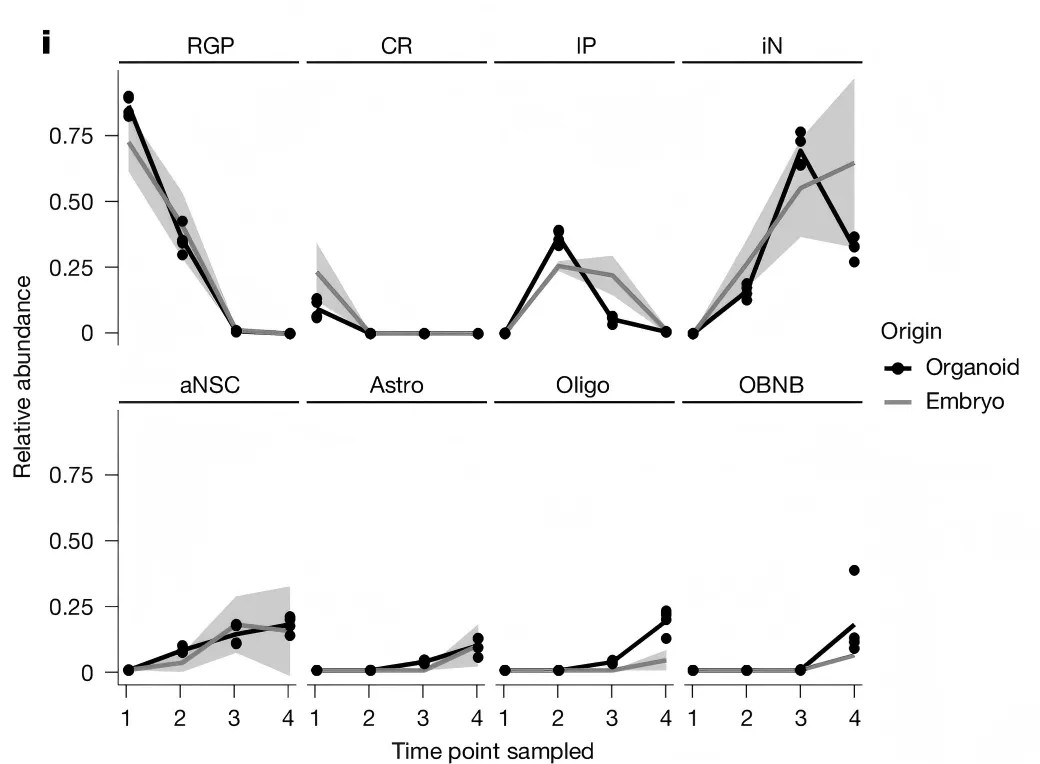
import osimport matplotlib.pyplot as pltfrom matplotlib.lines import Line2Dimport pandas as pd# 1. 自动创建“图表”文件夹output_dir = "图表"os.makedirs(output_dir, exist_ok=True)# 2. 读取同目录下的 data.xlsx 数据excel_path = "data.xlsx"df_org = pd.read_excel(excel_path, sheet_name="OrganoidData")df_emb = pd.read_excel(excel_path, sheet_name="EmbryoData")df_org_mean = (    df_org.groupby(["CellType", "TimePoint"])["Abundance"].mean().reset_index())# 3. 20种符合主流期刊标准的专业科研配色方案字典 (每行1种方案，含义附在行后)COLOR_PALETTES = {    1: {        "organoid": "#000000","embryo": "#7F7F7F",    },  # 经典黑灰 (Nature/Science单色常用风格)}# 选择配色方案 1selected_palette_id = 1current_palette = COLOR_PALETTES[selected_palette_id]color_organoid = current_palette["organoid"]color_embryo = current_palette["embryo"]# 4. 设置绘图全局属性cell_types = ["RGP", "CR", "IP", "iN", "aNSC", "Astro", "Oligo", "OBNB"]plt.rcParams["font.sans-serif"] = "DejaVu Sans"plt.rcParams["axes.edgecolor"] = "black"plt.rcParams["axes.linewidth"] = 1.0fig, axes = plt.subplots(2, 4, figsize=(10, 7.5), sharex=True, sharey=True)# 5. 遍历各个细胞类型并绘制子图for idx, cell_type in enumerate(cell_types):  r = idx // 4  c = idx % 4  ax = axes[r, c]  sub_emb = df_emb[df_emb["CellType"] == cell_type].sort_values("TimePoint")  sub_org_pts = df_org[df_org["CellType"] == cell_type]  sub_org_mean = df_org_mean[df_org_mean["CellType"] == cell_type].sort_values(      "TimePoint"  )  # (1) Embryo 折线及阴影  ax.plot(      sub_emb["TimePoint"],      sub_emb["Embryo_Mean"],      color=color_embryo,      linewidth=2.0,      zorder=2,  )  ax.fill_between(      sub_emb["TimePoint"],      sub_emb["Embryo_CI_Lower"],      sub_emb["Embryo_CI_Upper"],      color=color_embryo,      alpha=0.4,      zorder=1,      edgecolor="none",  )  # (2) Organoid 折线及散点  ax.plot(      sub_org_mean["TimePoint"],      sub_org_mean["Abundance"],      color=color_organoid,      linewidth=2.0,      zorder=3,  )  ax.scatter(      sub_org_pts["TimePoint"],      sub_org_pts["Abundance"],      color=color_organoid,      s=25,      zorder=4,  )  # 标题与刻度范围  ax.set_title(cell_type, fontsize=12, pad=6)  ax.set_xticks([1, 2, 3, 4])  ax.set_ylim(-0.05, 0.95)  ax.set_yticks([0.00, 0.25, 0.50, 0.75])  ax.tick_params(      axis="both",      which="major",      labelsize=11,      direction="out",      length=5,      width=1,  )  # 精确设定 Spine 端点，使左轴与顶线产生距离 gap  ax.spines["top"].set_visible(True)  ax.spines["top"].set_bounds(0.8, 4.2)  # 1. RGP  if cell_type == "RGP":    ax.spines["left"].set_visible(True)    ax.spines["left"].set_bounds(-0.02, 0.88)    ax.spines["bottom"].set_visible(False)    ax.spines["right"].set_visible(False)    ax.tick_params(        axis="x", which="both", bottom=False, top=False, labelbottom=False    )  # 2. CR, IP, iN  elif cell_type in ["CR", "IP", "iN"]:    ax.spines["left"].set_visible(False)    ax.spines["bottom"].set_visible(False)    ax.spines["right"].set_visible(False)    ax.tick_params(        axis="x", which="both", bottom=False, top=False, labelbottom=False    )    ax.tick_params(        axis="y", which="both", left=False, right=False, labelleft=False    )  # 3. aNSC  elif cell_type == "aNSC":    ax.spines["left"].set_visible(True)    ax.spines["left"].set_bounds(-0.02, 0.88)    ax.spines["bottom"].set_visible(True)    ax.spines["bottom"].set_bounds(0.8, 4.2)    ax.spines["right"].set_visible(False)  # 4. Astro, Oligo, OBNB  elif cell_type in ["Astro", "Oligo", "OBNB"]:    ax.spines["left"].set_visible(False)    ax.spines["bottom"].set_visible(True)    ax.spines["bottom"].set_bounds(0.8, 4.2)    ax.spines["right"].set_visible(False)    ax.tick_params(        axis="y", which="both", left=False, right=False, labelleft=False    )# 6. 全局文本标签fig.text(    0.5, 0.02, "Time point sampled", ha="center", va="center", fontsize=13)fig.text(    0.02,    0.5,    "Relative abundance",    ha="center",    va="center",    rotation="vertical",    fontsize=13,)fig.text(0.01, 0.96, "i", fontsize=16, fontweight="bold", ha="left", va="top")# 7. 全局图例legend_elements = [    Line2D(        [0],        [0],        color=color_organoid,        lw=2,        marker="o",        markersize=6,        label="Organoid",    ),    Line2D([0], [0], color=color_embryo, lw=2, label="Embryo"),]fig.legend(    handles=legend_elements,    title="Origin",    loc="center right",    bbox_to_anchor=(0.99, 0.55),    frameon=False,    title_fontsize=12,    fontsize=11,)# 8. 导出图像plt.tight_layout(rect=[0.04, 0.04, 0.86, 0.95])output_png_path = os.path.join(output_dir, "abundance_plot.png")plt.savefig(output_png_path, dpi=300)plt.close()print(f"导出图像完成: {output_png_path}")