R 代码|正刊地图|高阶地图制作|采样点地图

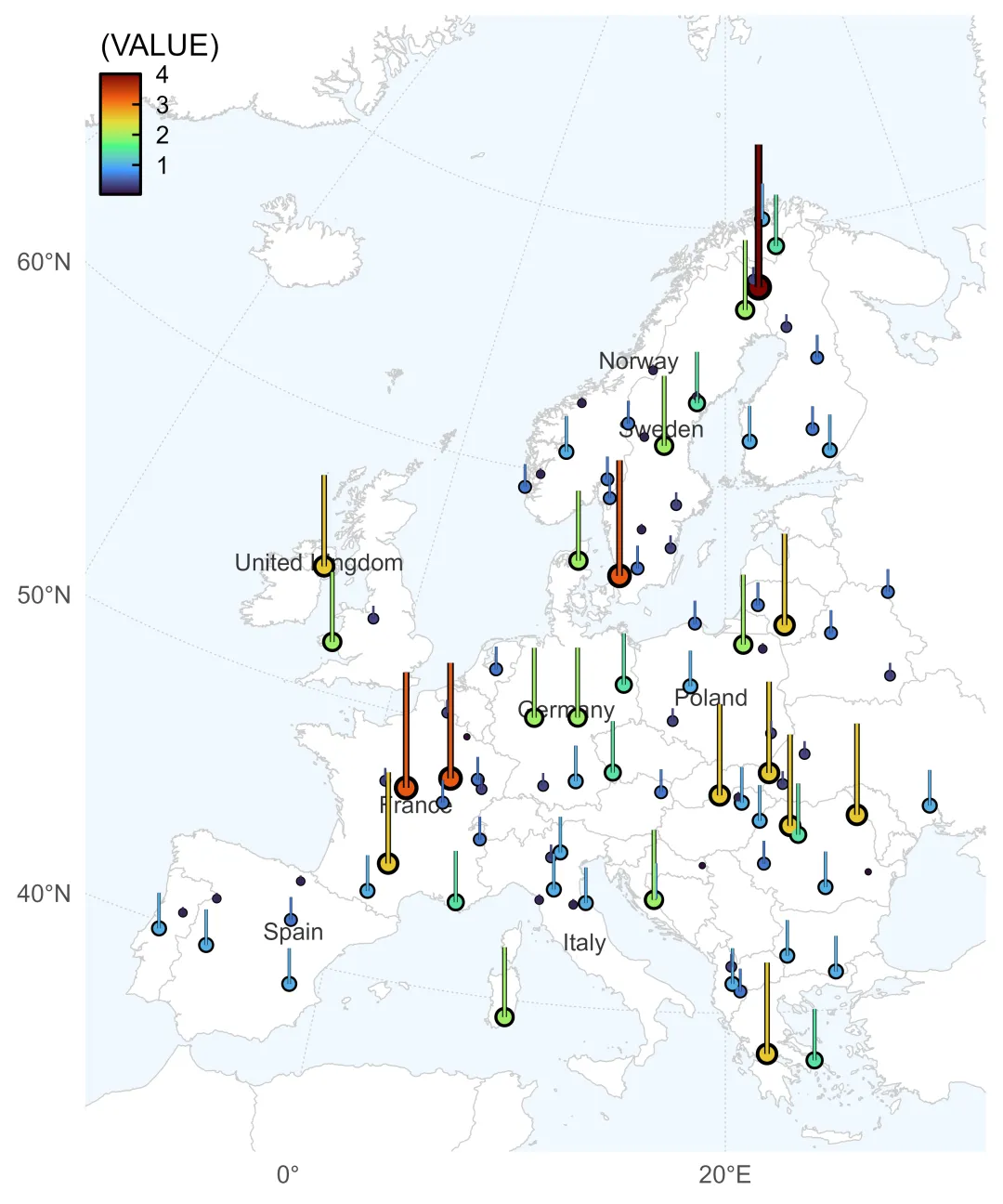
仿制一篇 Nature 论文地图（其附图 Extended Data Fig. 2 ）。易知，图中柱子高度代表某变量的数值大小——这或许比点的大小、颜色渐变更容易直接比较。

Pesticide residues alter taxonomic and functional biodiversity in soils

https://www.nature.com/articles/s41586-025-09991-z#Fig6

效果如下，

代码如下，

# =============================================================================# 欧洲三维地图可视化核心代码# 功能：获取欧洲空间数据、坐标处理、数据生成、地图绘制（伪 3D 效果）# 依赖包：ggplot2, dplyr, rnaturalearth, sf, geocn# =============================================================================# 1. 加载所需包 --------------------------------------------------------------library(ggplot2) # 可视化library(dplyr) # 数据处理library(rnaturalearth) # 地理边界数据library(sf) # 空间数据处理library(ggview) # 指定尺寸、分辨率预览# 安装 geocn# install.packages(#   "geocn",#   repos = c(#     "https://stscl.r-universe.dev",#     "https://cloud.r-project.org"#   ),#   dep = TRUE# )library(geocn)# 2. 获取欧洲地图数据 ---------------------------------------------------------# 世界地图world_country_sf <- geocn::load_world_country()# 获取欧洲国家地图（中等比例尺）# 裁剪范围europe_sf <- ne_countries(scale = "medium", returnclass = "sf") |>  filter(continent == "Europe") |>  filter(!name %in% c("Russia", "Turkey")) |>  st_crop(xmin = -10, xmax = 32, ymin = 36, ymax = 72) # 去除大部分海外岛屿europe_sf# 3. 提取欧洲边界并生成经纬度网格 ---------------------------------------------# 获取欧洲区域的边界框europe_bbox <- europe_sf |> st_bbox()# 调整边界范围，使欧洲居中显示lon_center <- mean(europe_bbox[c(1, 3)])lat_center <- mean(europe_bbox[c(2, 4)])# 4. 定义投影坐标系 -----------------------------------------------------------# GEOS投影（适合从侧面观看的3D效果，高度为同步卫星高度）# base_proj <- "+proj=geos +h=358000000 +ellps=WGS84 +no_defs"base_proj <- "+proj=laea +ellps=WGS84 +no_defs"# 设置投影中心为欧洲中心（经度15°，纬度50°）center_params <- paste0("+lon_0=", round(lon_center), " +lat_0=", round(lat_center))# 合并为完整投影定义full_proj <- paste(base_proj, center_params)# 5. 生成随机采样点及柱高数据 ------------------------------------------------# 增加采样点数量以适应更大区域sample_size <- 100set.seed(7) # 确保结果可复现# 在整个欧洲区域内随机采样sampled_points_sf <- st_sample(europe_sf, size = sample_size, type = "random") |>  st_as_sf()# 提取坐标并生成柱高数据sampled_data <- sampled_points_sf |>  st_coordinates() |>  as.data.frame() |>  rename(longitude = X, latitude = Y) |>  mutate(# bar_height = runif(n(), 0.2, 2.5) ^2, # 生成柱状图高度    bar_height = (rpois(n(), 5) / 5) ^2, # 生成柱状图高度# 添加国家信息（可选）    country = st_intersects(sampled_points_sf, europe_sf) |>      sapply(function(x) ifelse(length(x) > 0, europe_sf$name[x[1]], NA))  )# 6. 准备2D可视化数据 ---------------------------------------------------------# 调整投影中心参数，优化视角adjusted_proj <- paste(base_proj, "+lon_0=20 +lat_0=40") # 欧洲中心视角# 转换采样点到新投影坐标系magnification <- 1.5e5# 调整放大倍数transformed_data <- sampled_data |>  st_as_sf(coords = c("longitude", "latitude"), crs = "WGS84") |>  st_transform(crs = adjusted_proj) |>  st_coordinates() |>  as.data.frame() |>  mutate(# 放大柱高以便在2D图中清晰显示    bar_height = sampled_data$bar_height * magnification # 调整放大倍数  )# 转换欧洲地图到同一投影europe_reproj_sf <- europe_sf |> st_transform(adjusted_proj)# 7. 创建欧洲2D对比柱图 -------------------------------------------------------plot_2d_europe <- ggplot() +# 绘制世界国家边界  geom_sf(    data = world_country_sf,    color = "gray80",    fill = "gray100",    linewidth = 0.2  ) +# 若仅仅绘制欧洲国家边界# geom_sf(#   data = europe_reproj_sf,#   color = "gray80",#   fill = "gray100",#   linewidth = 0.2# ) +# 添加主要国家名称标签（避免标签重叠）  geom_sf_text(    data = europe_reproj_sf |>      filter(name %in% c("Germany", "France", "United Kingdom", "Italy","Spain", "Poland", "Sweden", "Norway"      )),    aes(label = name),    family = "sans",    color = "gray20",    size = 3,    check_overlap = TRUE  ) +# 绘制采样点（大小和颜色根据柱高变化）  geom_point(    data = transformed_data,    aes(x = X, y = Y, size = bar_height * 3),    color = "grey0",# alpha = 0.8  ) +  geom_point(    data = transformed_data,    aes(x = X, y = Y, size = bar_height, color = bar_height / magnification),# alpha = 0.6  ) +# 绘制柱状图线段  geom_segment(    data = transformed_data,    aes(      x = X,      y = Y,      xend = X,      yend = Y + bar_height,      linewidth = bar_height * 3    ),    color = "grey0"  ) +  geom_segment(    data = transformed_data,    aes(      x = X,      y = Y,      xend = X,      yend = Y + bar_height,      color = bar_height / magnification,      linewidth = bar_height    )  ) +# 颜色和尺寸比例尺设置  scale_color_viridis_c(    option = "H", # A~H    direction = 1,    name = "(VALUE)"  ) +# scale_color_distiller(#   palette = "RdYlBu",#   direction = -1,#   name = "(VALUE)"# ) +  scale_size_continuous(guide = "none", range = c(0.4, 4)) +  scale_linewidth_continuous(guide = "none", range = c(0.3, 1.3)) +  labs(x = NULL, y = NULL) +# 坐标系设置  coord_sf(    crs = adjusted_proj,    xlim = st_bbox(europe_reproj_sf)[c("xmin", "xmax")] * 1,    ylim = st_bbox(europe_reproj_sf)[c("ymin", "ymax")] * 1.1, # 增加5%边距# clip = "off"  ) +# 主题设置  theme_minimal(base_line_size = 0.4) +# theme_classic(base_line_size = 0.4) +# theme_linedraw(base_rect_size = 0.3, base_line_size = 0.4) +  theme(# plot.margin = margin(t = 5, b = 0, l = 0, r = 0),    panel.background = element_rect(color = NA, fill = "aliceblue", linewidth = 0),    panel.grid.major = element_line(color = "grey80", linewidth = 0.2, linetype = 3),    legend.position = c(0, 1),    legend.justification = c(0, 1),    legend.background = element_blank(),    legend.key.width = unit(1, "line"),    legend.key.height = unit(0.6, "line"),# legend.box.background = element_rect(color = NA, fill = alpha("grey100", 1)),    legend.frame = element_rect(color = "black"),    legend.ticks = element_line(color = "black"),    legend.ticks.length = unit(c(3, 0), "pt")  )# 8. 展示2D地图 --------------------------------------------------------------plot_2d_europe + ggview::canvas(5, 6, dpi = 600)