MATLAB 和 Python 画带两端尖角的colorbar:以极坐标散点密度图为例(含代码)

引言

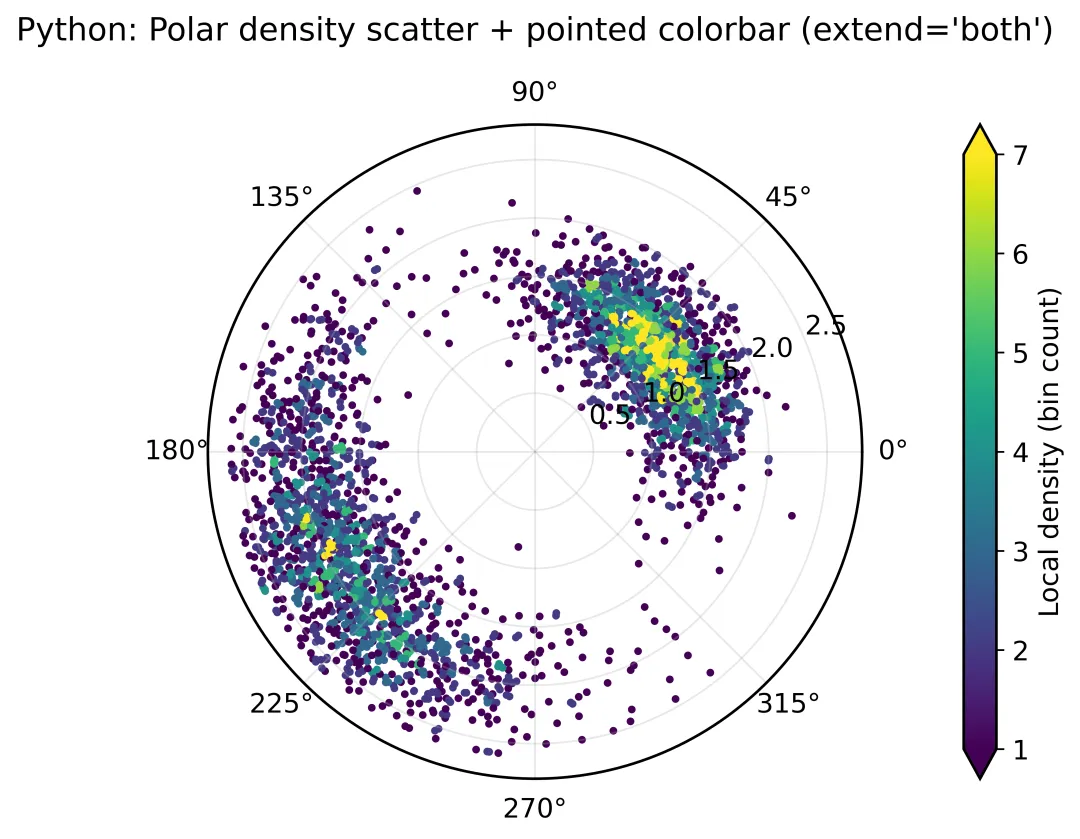
很多论文图里 colorbar 做成普通矩形，会把“超量程/溢出”的信息藏起来，读者很难一眼判断是否存在极端值。两端带尖角的 colorbar（类似 extend）是一个非常强的视觉信号：它明确告诉读者当前颜色范围是裁剪过的，低于下限或高于上限的数据并没有消失，只是被归入尖角端的“溢出区”。本文用一个极坐标散点密度图做例子：把极坐标点(θ,r) 转为 (x,y)后，用二维分箱计数快速得到局部密度，再将密度映射为散点颜色。Python 中只需 colorbar 的 extend='both' 就能得到两端尖角；MATLAB 则可以用 colorbar 后在其轴上叠加上下两个三角形 patch 实现同样效果。两段代码都采用分位数裁剪色标范围，让尖角真正表达“超范围”的数据含义，适合密度、误差、强度等任何可能出现极端值的科研可视化场景。

解决办法

Python 代码（极坐标密度散点 + 尖角 colorbar）

plt.colorbar(..., extend='both')直接出两端尖角。

MATLAB 代码（极坐标密度散点 + 尖角 colorbar）

MATLAB 本身 colorbar 没有“一行命令两端尖角”的通用接口，所以这里用 patch 在 colorbar 上画两个三角形实现。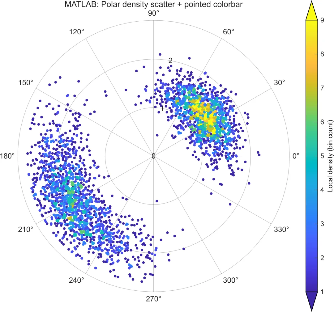

具体代码

具体Python如下：

import numpy as np

import pandas as pd

import matplotlib.pyplot as plt

#1) 生成演示数据（替换成你的 theta/r 也行）

rng = np.random.default_rng(2)

n = 3000

theta1 = rng.vonmises(mu=np.deg2rad(40),  kappa=6, size=n//2)

r1 = np.clip(rng.normal(1.4, 0.25, size=n//2), 0.1, 2.4)

theta2 = rng.vonmises(mu=np.deg2rad(210), kappa=4, size=n//2)

r2 = np.clip(rng.normal(2.0, 0.30, size=n//2), 0.1, 2.6)

theta = np.concatenate([theta1, theta2]) % (2*np.pi)

r = np.concatenate([r1, r2])

x = r*np.cos(theta)

y = r*np.sin(theta)

# ========== 2) 快速密度：二维分箱计数 ==========

nb = 80

H, xedges, yedges = np.histogram2d(x, y, bins=nb)

ix = np.clip(np.searchsorted(xedges, x, side="right") - 1, 0, nb-1)

iy = np.clip(np.searchsorted(yedges, y, side="right") - 1, 0, nb-1)

dens = H[ix, iy]

# 裁色标范围到分位数，制造“溢出” -> 让尖角有意义

vmin = np.quantile(dens, 0.05)

vmax = np.quantile(dens, 0.95)

# ========== 3) 极坐标散点密度图 ==========

plt.rcParams.update({

    "font.size": 12,

    "axes.linewidth": 1.2,

    "figure.facecolor": "white"

})

fig = plt.figure(figsize=(7.0, 5.4))

ax = fig.add_subplot(111, projection="polar")

sc = ax.scatter(theta, r, c=dens, s=12, cmap="viridis",

                vmin=vmin, vmax=vmax, linewidths=0)

ax.set_title("Python: Polar density scatter + pointed colorbar (extend='both')", pad=18)

ax.set_rmax(2.8)

ax.grid(True, alpha=0.3)

cb = fig.colorbar(sc, ax=ax, pad=0.10, fraction=0.06, extend="both")

cb.set_label("Local density (bin count)")

fig.tight_layout()

fig.savefig("PY_polar_density_pointed.png", dpi=600, bbox_inches="tight")

plt.close(fig)

具体Matlab代码如下：

%% polar_density_pointed_colorbar_fix.m

clear; clc; close all;

rng(2);

n = 3000;

% --- 1) 造数据（两团方向聚集） ---

theta1 = deg2rad(40)  + randn(n/2,1) * 0.35;

theta2 = deg2rad(210) + randn(n/2,1) * 0.45;

theta = mod([theta1; theta2], 2*pi);

r1 = min(max(1.4 + 0.25*randn(n/2,1), 0.1), 2.4);

r2 = min(max(2.0 + 0.30*randn(n/2,1), 0.1), 2.6);

r  = [r1; r2];

x = r .* cos(theta);

y = r .* sin(theta);

% --- 2) 二维分箱密度（用 histcounts2，拿到每个点的bin） ---

nb = 80;

xe = linspace(min(x), max(x), nb+1);

ye = linspace(min(y), max(y), nb+1);

% binX/binY: 每个点落在哪个格子；0 表示落在边界外（极少）

[N,~,~,binX,binY] = histcounts2(x, y, xe, ye);

% 把边界外(=0)的点“夹”回边界内，避免全被过滤

binX(binX==0) = 1;

binY(binY==0) = 1;

binX(binX>nb) = nb;

binY(binY>nb) = nb;

dens = N(sub2ind(size(N), binX, binY));  % 注意 histcounts2 输出 N 的维度是 (nb x nb)

% 为了显示尖角：裁色标范围到分位数

vmin = quantile(dens, 0.05);

vmax = quantile(dens, 0.95);

% --- 3) 极坐标散点密度图 ---

fig = figure('Color','w','Position',[200 100 820 600]);

pax = polaraxes(fig); hold(pax,'on');

pax.RLim = [0 2.8];

pax.GridAlpha = 0.30;

title(pax, 'MATLAB: Polar density scatter + pointed colorbar');

polarscatter(pax, theta, r, 12, dens, 'filled');

colormap(pax, parula(256));

caxis(pax, [vmin vmax]);

% --- 4) colorbar + 两端尖角（在 colorbar 上叠加三角形） ---

cb = colorbar(pax);

cb.Label.String = 'Local density (bin count)';

drawnow;

cbpos = cb.Position;

ax2 = axes('Parent', fig, 'Position', cbpos, ...

    'Color','none', 'XLim',[0 1], 'YLim',[0 1], ...

    'XTick',[], 'YTick',[], 'Box','off');

ax2.HitTest = 'off';

th = 0.07;                 % 三角高度（占 colorbar 高度比例）

cm = colormap(pax);

lowc  = cm(1,:);

highc = cm(end,:);

patch(ax2, [0 1 0.5], [0 0 -th], lowc,  'EdgeColor','k','LineWidth',0.8,'Clipping','off');

patch(ax2, [0 1 0.5], [1 1 1+th], highc, 'EdgeColor','k','LineWidth',0.8,'Clipping','off');

uistack(cb, 'top');

exportgraphics(fig, 'MATLAB_polar_density_pointed.png', 'Resolution', 600);

特别声明：

以上代码与文案均为网上资料整合而成，仅供广大同行们参考学习，如有侵权请联系删除。

如有其他需要，欢迎关注我的咸鱼号:pfc小姐姐