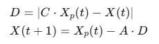
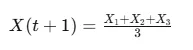
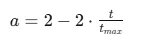
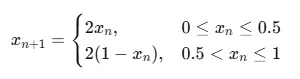
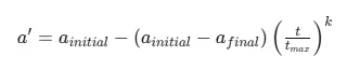
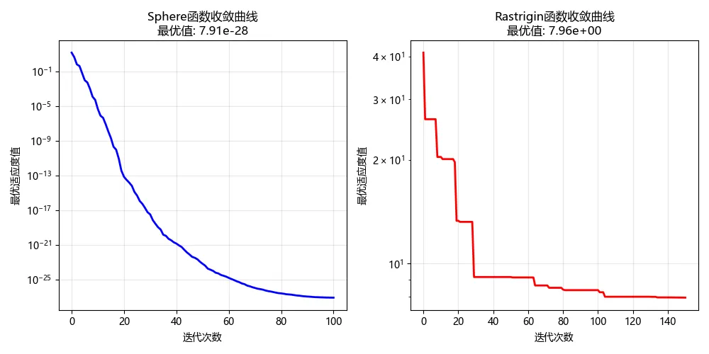
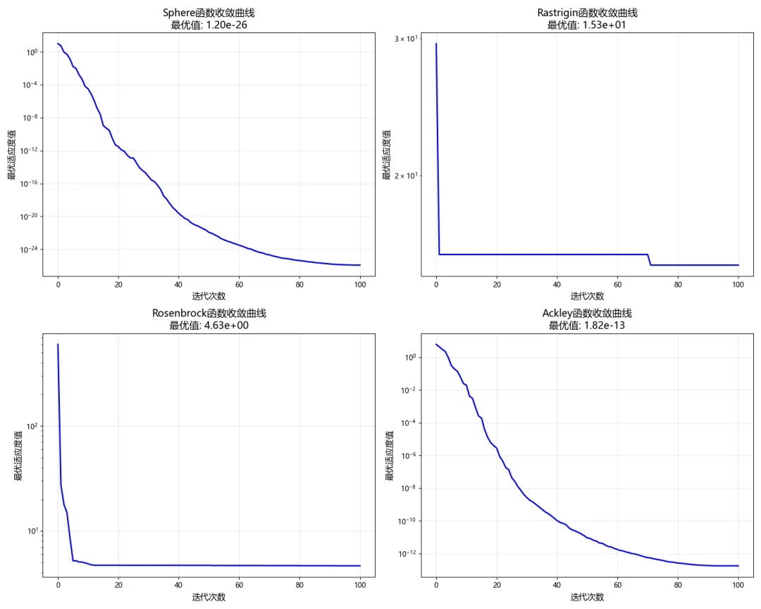
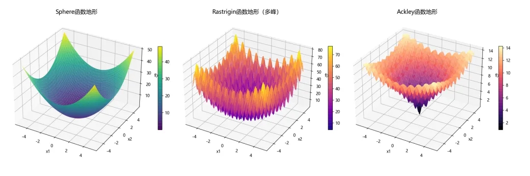
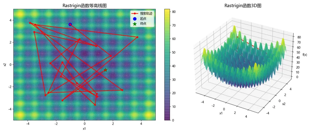
import numpy as npimport matplotlib.pyplot as pltfrom mpl_toolkits.mplot3d import Axes3Dimport warningswarnings.filterwarnings('ignore')import matplotlib.pyplot as pltimport matplotlib.font_manager as fmplt.rcParams['font.sans-serif'] = ['Microsoft YaHei', 'SimHei', 'Arial Unicode MS', 'DejaVu Sans']plt.rcParams['axes.unicode_minus'] = Falseclass AdaptiveCooperativeGWO: """自适应协同灰狼优化算法""" def __init__(self, obj_func, dim, lb, ub, max_iter=100, pop_size=30): """ 初始化参数 obj_func: 目标函数(最小化问题) dim: 变量维度 lb: 下界 ub: 上界 max_iter: 最大迭代次数 pop_size: 种群大小 """ self.obj_func = obj_func self.dim = dim self.lb = np.array(lb) if isinstance(lb, list) else np.ones(dim) * lb self.ub = np.array(ub) if isinstance(ub, list) else np.ones(dim) * ub self.max_iter = max_iter self.pop_size = pop_size # 存储收敛历史 self.convergence_curve = [] def tent_map_initialization(self): """改进的Tent混沌映射初始化种群""" # 产生混沌序列 p = np.random.rand(self.pop_size, self.dim) for i in range(1, self.pop_size): for j in range(self.dim): if p[i - 1, j] < 0.5: p[i, j] = 2 * p[i - 1, j] else: p[i, j] = 2 * (1 - p[i - 1, j]) # 映射到搜索空间 positions = self.lb + p * (self.ub - self.lb) return positions def nonlinear_adaptive_a(self, t): """非线性自适应收敛因子""" a_initial = 2 a_final = 0 k = 2 # 调节系数 # 非线性自适应收敛因子公式 a = a_initial - (a_initial - a_final) * (t / self.max_iter) ** (1 / k) return a def alpha_local_search(self, alpha_pos, delta_pos, alpha_score): """α狼局部搜索""" # 在α狼周围基于与δ狼的距离进行局部搜索 new_alpha = alpha_pos.copy() for i in range(self.dim): # 搜索范围定义为α与δ之间的距离 search_range = abs(alpha_pos[i] - delta_pos[i]) * 0.1 # 在范围内随机搜索 step = np.random.uniform(-search_range, search_range) new_alpha[i] = alpha_pos[i] + step # 边界处理 new_alpha[i] = np.clip(new_alpha[i], self.lb[i], self.ub[i]) # 评估新位置 new_score = self.obj_func(new_alpha) # 如果找到更优位置,则更新 if new_score < alpha_score: return new_alpha, new_score else: return alpha_pos, alpha_score def optimize(self): """执行优化""" # Tent混沌映射初始化种群 positions = self.tent_map_initialization() # 初始化个体历史最优 personal_best_pos = positions.copy() personal_best_score = np.array([self.obj_func(p) for p in positions]) # 初始化全局最优(α、β、δ) scores = personal_best_score.copy() sorted_indices = np.argsort(scores) alpha_pos = positions[sorted_indices[0]].copy() alpha_score = scores[sorted_indices[0]] beta_pos = positions[sorted_indices[1]].copy() beta_score = scores[sorted_indices[1]] delta_pos = positions[sorted_indices[2]].copy() delta_score = scores[sorted_indices[2]] # 记录每次迭代的最优值 self.convergence_curve = [alpha_score] # 主循环 for t in range(self.max_iter): # 非线性自适应收敛因子 a = self.nonlinear_adaptive_a(t) for i in range(self.pop_size): # 对每个灰狼个体,根据α、β、δ更新位置 new_pos = np.zeros(self.dim) for j in range(self.dim): # 根据α狼更新 r1, r2 = np.random.rand(2) A1 = 2 * a * r1 - a C1 = 2 * r2 D_alpha = abs(C1 * alpha_pos[j] - positions[i, j]) X1 = alpha_pos[j] - A1 * D_alpha # 根据β狼更新 r1, r2 = np.random.rand(2) A2 = 2 * a * r1 - a C2 = 2 * r2 D_beta = abs(C2 * beta_pos[j] - positions[i, j]) X2 = beta_pos[j] - A2 * D_beta # 根据δ狼更新 r1, r2 = np.random.rand(2) A3 = 2 * a * r1 - a C3 = 2 * r2 D_delta = abs(C3 * delta_pos[j] - positions[i, j]) X3 = delta_pos[j] - A3 * D_delta # 融合三只头狼的信息(协同机制) # 同时结合个体历史最优(记忆功能) w1, w2, w3, w4 = 0.3, 0.3, 0.3, 0.1 # 权重系数 new_pos[j] = w1 * X1 + w2 * X2 + w3 * X3 + w4 * personal_best_pos[i, j] # 边界处理 new_pos = np.clip(new_pos, self.lb, self.ub) # 评估新位置 new_score = self.obj_func(new_pos) # 更新个体历史最优 if new_score < personal_best_score[i]: personal_best_pos[i] = new_pos.copy() personal_best_score[i] = new_score # 更新位置 positions[i] = new_pos.copy() # 更新α、β、δ if new_score < alpha_score: delta_pos = beta_pos.copy() delta_score = beta_score beta_pos = alpha_pos.copy() beta_score = alpha_score alpha_pos = new_pos.copy() alpha_score = new_score elif new_score < beta_score: delta_pos = beta_pos.copy() delta_score = beta_score beta_pos = new_pos.copy() beta_score = new_score elif new_score < delta_score: delta_pos = new_pos.copy() delta_score = new_score # α狼局部搜索(每10次迭代进行一次) if t % 10 == 0 and t > 0: alpha_pos, alpha_score = self.alpha_local_search(alpha_pos, delta_pos, alpha_score) # 记录收敛曲线 self.convergence_curve.append(alpha_score) # 输出进度 if (t + 1) % 20 == 0: print(f'迭代次数: {t + 1}, 当前最优值: {alpha_score:.6e}') return alpha_pos, alpha_score, self.convergence_curve# 定义测试函数def sphere(x): """Sphere函数,单峰,最小值0在(0,0,...,0)""" return np.sum(x ** 2)def rastrigin(x): """Rastrigin函数,多峰,有大量局部最优,最小值0在(0,0,...,0)""" x = np.array(x) # 确保输入是numpy数组 dim = len(x) return 10 * dim + np.sum(x ** 2 - 10 * np.cos(2 * np.pi * x))def rosenbrock(x): """Rosenbrock函数,单峰但路径狭窄,最小值0在(1,1,...,1)""" x = np.array(x) # 确保输入是numpy数组 dim = len(x) return np.sum(100 * (x[1:] - x[:-1] ** 2) ** 2 + (x[:-1] - 1) ** 2)def ackley(x): """Ackley函数,多峰,最小值0在(0,0,...,0)""" x = np.array(x) # 确保输入是numpy数组 dim = len(x) sum1 = np.sum(x ** 2) sum2 = np.sum(np.cos(2 * np.pi * x)) return -20 * np.exp(-0.2 * np.sqrt(sum1 / dim)) - np.exp(sum2 / dim) + 20 + np.edef plot_convergence_comparison(): """比较不同函数的收敛曲线""" np.random.seed(42) dim = 5 max_iter = 100 pop_size = 30 functions = [sphere, rastrigin, rosenbrock, ackley] func_names = ['Sphere函数', 'Rastrigin函数', 'Rosenbrock函数', 'Ackley函数'] bounds = [(-5.12, 5.12), (-5.12, 5.12), (-2.048, 2.048), (-5, 5)] fig, axes = plt.subplots(2, 2, figsize=(15, 12)) axes = axes.flatten() for idx, (func, name, bound) in enumerate(zip(functions, func_names, bounds)): lb = [bound[0]] * dim ub = [bound[1]] * dim print(f"\n正在优化 {name}...") acgwo = AdaptiveCooperativeGWO(func, dim, lb, ub, max_iter, pop_size) best_pos, best_score, convergence = acgwo.optimize() axes[idx].plot(convergence, 'b-', linewidth=2) axes[idx].set_xlabel('迭代次数', fontsize=12) axes[idx].set_ylabel('最优适应度值', fontsize=12) axes[idx].set_title(f'{name}收敛曲线\n最优值: {best_score:.2e}', fontsize=14) axes[idx].set_yscale('log') axes[idx].grid(True, alpha=0.3) plt.tight_layout() plt.savefig('convergence_comparison.png', dpi=300, bbox_inches='tight') plt.show()def plot_3d_landscape(): """绘制三维函数地形""" fig = plt.figure(figsize=(18, 6)) # 生成网格数据 x = np.linspace(-5, 5, 100) y = np.linspace(-5, 5, 100) X, Y = np.meshgrid(x, y) # 计算函数值 - 将网格点转换为适合函数调用的格式 Z_sphere = X ** 2 + Y ** 2 # Rastrigin函数 Z_rastrigin = np.zeros_like(X) for i in range(X.shape[0]): for j in range(X.shape[1]): Z_rastrigin[i, j] = rastrigin([X[i, j], Y[i, j]]) # Ackley函数 Z_ackley = np.zeros_like(X) for i in range(X.shape[0]): for j in range(X.shape[1]): Z_ackley[i, j] = ackley([X[i, j], Y[i, j]]) # Sphere函数 ax1 = fig.add_subplot(131, projection='3d') surf1 = ax1.plot_surface(X, Y, Z_sphere, cmap='viridis', alpha=0.9) ax1.set_title('Sphere函数地形', fontsize=14) ax1.set_xlabel('x1') ax1.set_ylabel('x2') ax1.set_zlabel('f(x)') plt.colorbar(surf1, ax=ax1, shrink=0.5) # Rastrigin函数 ax2 = fig.add_subplot(132, projection='3d') surf2 = ax2.plot_surface(X, Y, Z_rastrigin, cmap='plasma', alpha=0.9) ax2.set_title('Rastrigin函数地形(多峰)', fontsize=14) ax2.set_xlabel('x1') ax2.set_ylabel('x2') ax2.set_zlabel('f(x)') plt.colorbar(surf2, ax=ax2, shrink=0.5) # Ackley函数 ax3 = fig.add_subplot(133, projection='3d') surf3 = ax3.plot_surface(X, Y, Z_ackley, cmap='magma', alpha=0.9) ax3.set_title('Ackley函数地形', fontsize=14) ax3.set_xlabel('x1') ax3.set_ylabel('x2') ax3.set_zlabel('f(x)') plt.colorbar(surf3, ax=ax3, shrink=0.5) plt.tight_layout() plt.savefig('function_landscapes.png', dpi=300, bbox_inches='tight') plt.show()def plot_strategy_animation(): """模拟搜索过程的动态图""" np.random.seed(42) # 生成二维搜索空间 x = np.linspace(-5, 5, 200) y = np.linspace(-5, 5, 200) X, Y = np.meshgrid(x, y) # 计算Z值 Z = np.zeros_like(X) for i in range(X.shape[0]): for j in range(X.shape[1]): Z[i, j] = rastrigin([X[i, j], Y[i, j]]) # 创建图形 fig = plt.figure(figsize=(15, 6)) # 左图:等高线图 ax1 = fig.add_subplot(121) contour = ax1.contourf(X, Y, Z, levels=50, cmap='viridis', alpha=0.8) plt.colorbar(contour, ax=ax1) ax1.set_title('Rastrigin函数等高线图', fontsize=14) ax1.set_xlabel('x1') ax1.set_ylabel('x2') # 右图:3D图 ax2 = fig.add_subplot(122, projection='3d') surf = ax2.plot_surface(X, Y, Z, cmap='viridis', alpha=0.8) ax2.set_title('Rastrigin函数3D图', fontsize=14) ax2.set_xlabel('x1') ax2.set_ylabel('x2') ax2.set_zlabel('f(x)') # 模拟搜索轨迹 n_steps = 20 positions = np.random.uniform(-4, 4, (n_steps, 2)) # 计算每个位置的高度 heights = np.array([rastrigin([p[0], p[1]]) for p in positions]) # 在等高线图上绘制搜索轨迹 ax1.plot(positions[:, 0], positions[:, 1], 'r.-', linewidth=2, markersize=10, label='搜索轨迹') ax1.scatter(positions[0, 0], positions[0, 1], c='blue', s=100, marker='o', label='起点') ax1.scatter(positions[-1, 0], positions[-1, 1], c='green', s=150, marker='*', label='终点') ax1.legend() # 在3D图上绘制搜索轨迹 ax2.plot(positions[:, 0], positions[:, 1], heights, 'r.-', linewidth=2, markersize=10) ax2.scatter(positions[0, 0], positions[0, 1], heights[0], c='blue', s=100, marker='o') ax2.scatter(positions[-1, 0], positions[-1, 1], heights[-1], c='green', s=150, marker='*') plt.tight_layout() plt.savefig('search_trajectory.png', dpi=300, bbox_inches='tight') plt.show()def main(): """主函数""" print("=" * 60) print("自适应协同灰狼优化算法演示") print("=" * 60) # 示例1:求解Sphere函数(低维) print("\n【示例1】求解Sphere函数(5维)") dim = 5 acgwo = AdaptiveCooperativeGWO(sphere, dim, -5.12, 5.12, max_iter=100, pop_size=30) best_pos, best_score, convergence = acgwo.optimize() print(f"最优解位置: {best_pos}") print(f"最优函数值: {best_score:.2e}") # 绘制收敛曲线 plt.figure(figsize=(10, 5)) plt.subplot(1, 2, 1) plt.plot(convergence, 'b-', linewidth=2) plt.xlabel('迭代次数') plt.ylabel('最优适应度值') plt.title(f'Sphere函数收敛曲线\n最优值: {best_score:.2e}') plt.yscale('log') plt.grid(True, alpha=0.3) # 示例2:求解Rastrigin函数 print("\n【示例2】求解Rastrigin函数(5维,多峰函数)") acgwo2 = AdaptiveCooperativeGWO(rastrigin, dim, -5.12, 5.12, max_iter=150, pop_size=40) best_pos2, best_score2, convergence2 = acgwo2.optimize() print(f"最优解位置: {best_pos2}") print(f"最优函数值: {best_score2:.2e}") plt.subplot(1, 2, 2) plt.plot(convergence2, 'r-', linewidth=2) plt.xlabel('迭代次数') plt.ylabel('最优适应度值') plt.title(f'Rastrigin函数收敛曲线\n最优值: {best_score2:.2e}') plt.yscale('log') plt.grid(True, alpha=0.3) plt.tight_layout() plt.savefig('basic_convergence.png', dpi=300, bbox_inches='tight') plt.show() # 绘制更多可视化 print("\n生成可视化图表...") print("1. 绘制多函数收敛对比图...") plot_convergence_comparison() print("2. 绘制函数地形图...") plot_3d_landscape() print("3. 绘制搜索轨迹图...") plot_strategy_animation()if __name__ == "__main__": main()