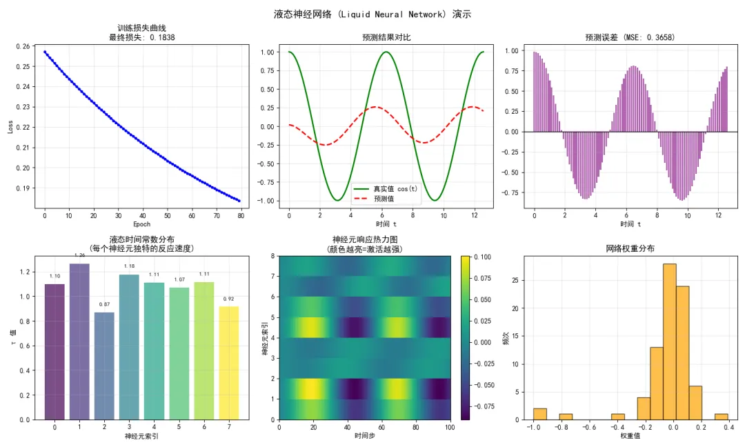
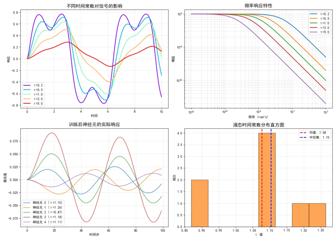
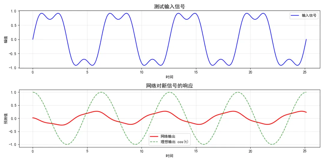
import numpy as npimport matplotlib.pyplot as pltimport timeplt.rcParams['font.sans-serif'] = ['SimHei', 'Microsoft YaHei', 'DejaVu Sans']plt.rcParams['axes.unicode_minus'] = False# 设置随机种子np.random.seed(42)# ======================# 1. 数据准备# ======================def generate_data(): """生成训练数据:从sin(t)预测cos(t)""" t = np.linspace(0, 4 * np.pi, 100) X = np.sin(t).reshape(-1, 1) Y = np.cos(t).reshape(-1, 1) return t, X, Yt, X, Y = generate_data()print(f"数据形状 - X: {X.shape}, Y: {Y.shape}")# ======================# 2. 液态神经元层# ======================class LiquidLayer: """液态神经元层""" def __init__(self, input_size, hidden_size, dt=0.1): self.input_size = input_size self.hidden_size = hidden_size self.dt = dt # 初始化参数 self.W_in = np.random.randn(hidden_size, input_size) * 0.1 self.W_h = np.random.randn(hidden_size, hidden_size) * 0.1 self.bias = np.zeros(hidden_size) self.log_tau = np.random.randn(hidden_size) * 0.1 @property def tau(self): return np.exp(self.log_tau) + 0.1 def forward(self, x, return_all=False): """ 前向传播 x: 输入序列 [seq_len, input_size] """ seq_len = x.shape[0] h = np.zeros(self.hidden_size) h_seq = [] for t in range(seq_len): x_t = x[t] # 液态神经元动力学 pre_act = np.dot(self.W_in, x_t) + np.dot(self.W_h, h) + self.bias dh = (-h + np.tanh(pre_act)) / self.tau h = h + self.dt * dh h_seq.append(h.copy()) h_seq = np.array(h_seq) if return_all: return h_seq else: return h_seq[-1] # 只返回最后一个时间步# ======================# 3. 液态神经网络# ======================class LiquidNeuralNetwork: """液态神经网络""" def __init__(self, input_size=1, hidden_size=10, output_size=1, lr=0.01): self.hidden_size = hidden_size self.lr = lr # 液态层 self.liquid = LiquidLayer(input_size, hidden_size) # 输出层 self.W_out = np.random.randn(output_size, hidden_size) * 0.1 self.b_out = np.zeros(output_size) self.loss_history = [] def forward(self, x): """前向传播 - 返回最后一个时间步的预测""" h_last = self.liquid.forward(x, return_all=False) y_pred = np.dot(self.W_out, h_last) + self.b_out return y_pred, h_last def forward_all(self, x): """前向传播 - 返回所有时间步的隐藏状态""" h_seq = self.liquid.forward(x, return_all=True) return h_seq def compute_loss(self, y_pred, y_true): """计算损失""" return 0.5 * np.mean((y_pred - y_true) ** 2) def train_step(self, x, y_true): """单步训练""" # 保存当前参数 W_out_old = self.W_out.copy() b_out_old = self.b_out.copy() log_tau_old = self.liquid.log_tau.copy() # 前向传播 y_pred, h_last = self.forward(x) loss = self.compute_loss(y_pred, y_true) # 计算输出层梯度(解析梯度) error = y_pred - y_true # [output_size] grad_W_out = np.outer(error, h_last) # [output_size, hidden_size] grad_b_out = error # [output_size] # 更新输出层 self.W_out -= self.lr * grad_W_out self.b_out -= self.lr * grad_b_out # 计算液态层梯度(数值梯度) eps = 1e-4 # 对每个液态时间常数计算梯度 for i in range(self.hidden_size): # 保存原始值 original_tau = self.liquid.log_tau[i] # 正向扰动 self.liquid.log_tau[i] = original_tau + eps y_pred_plus, _ = self.forward(x) loss_plus = self.compute_loss(y_pred_plus, y_true) # 负向扰动 self.liquid.log_tau[i] = original_tau - eps y_pred_minus, _ = self.forward(x) loss_minus = self.compute_loss(y_pred_minus, y_true) # 恢复原始值 self.liquid.log_tau[i] = original_tau # 计算梯度并更新 grad_tau = (loss_plus - loss_minus) / (2 * eps) self.liquid.log_tau[i] -= self.lr * grad_tau * 0.1 return loss def train(self, X, Y, epochs=100): """训练模型""" print("开始训练...") start_time = time.time() for epoch in range(epochs): # 对每个时间点进行训练(使用最后一个点的目标值) total_loss = 0 for i in range(len(X)): x_seq = X[:i + 1] # 使用到当前时间点的所有历史 y_true = Y[i] # 当前时间点的目标值 loss = self.train_step(x_seq, y_true) total_loss += loss avg_loss = total_loss / len(X) self.loss_history.append(avg_loss) if (epoch + 1) % 20 == 0: print(f'Epoch [{epoch + 1}/{epochs}], Loss: {avg_loss:.6f}') train_time = time.time() - start_time print(f"训练完成,用时: {train_time:.2f} 秒") return self.loss_history def predict(self, X): """预测整个序列""" predictions = [] for i in range(len(X)): x_seq = X[:i + 1] y_pred, _ = self.forward(x_seq) predictions.append(y_pred[0]) return np.array(predictions) def get_neuron_responses(self, X): """获取所有神经元的响应""" h_seq = self.forward_all(X) return h_seq# ======================# 4. 训练模型# ======================print("\n" + "=" * 50)print("创建液态神经网络...")model = LiquidNeuralNetwork( input_size=1, hidden_size=8, # 8个神经元,足够快 output_size=1, lr=0.005 # 学习率)# 训练loss_history = model.train(X, Y, epochs=80)# ======================# 5. 预测# ======================Y_pred = model.predict(X)# ======================# 6. 可视化# ======================fig, axes = plt.subplots(2, 3, figsize=(15, 9))# 图1: 训练损失ax1 = axes[0, 0]ax1.plot(loss_history, 'b-', linewidth=2, marker='o', markersize=3)ax1.set_title(f'训练损失曲线\n最终损失: {loss_history[-1]:.4f}', fontsize=12)ax1.set_xlabel('Epoch')ax1.set_ylabel('Loss')ax1.grid(True, alpha=0.3)# 图2: 预测 vs 真实值ax2 = axes[0, 1]ax2.plot(t, Y.flatten(), 'g-', label='真实值 cos(t)', linewidth=2)ax2.plot(t, Y_pred, 'r--', label='预测值', linewidth=2)ax2.set_title('预测结果对比', fontsize=12)ax2.set_xlabel('时间 t')ax2.legend()ax2.grid(True, alpha=0.3)# 图3: 预测误差ax3 = axes[0, 2]error = Y.flatten() - Y_predmse = np.mean(error ** 2)ax3.bar(t, error, width=0.1, color='purple', alpha=0.6)ax3.set_title(f'预测误差 (MSE: {mse:.4f})', fontsize=12)ax3.set_xlabel('时间 t')ax3.axhline(y=0, color='black', linestyle='-', linewidth=1)ax3.grid(True, alpha=0.3)# 图4: 液态时间常数ax4 = axes[1, 0]tau_values = model.liquid.taucolors = plt.cm.viridis(np.linspace(0, 1, len(tau_values)))bars = ax4.bar(range(len(tau_values)), tau_values, color=colors, alpha=0.7)ax4.set_title('液态时间常数分布\n(每个神经元独特的反应速度)', fontsize=12)ax4.set_xlabel('神经元索引')ax4.set_ylabel('τ 值')ax4.grid(True, alpha=0.3)# 在每个柱子上标出数值for i, (bar, val) in enumerate(zip(bars, tau_values)): ax4.text(bar.get_x() + bar.get_width() / 2, bar.get_height() + 0.05, f'{val:.2f}', ha='center', va='bottom', fontsize=8)# 图5: 神经元响应热力图ax5 = axes[1, 1]neuron_responses = model.get_neuron_responses(X)im = ax5.imshow(neuron_responses.T, aspect='auto', cmap='viridis', extent=[0, len(t), 0, model.hidden_size])ax5.set_title('神经元响应热力图\n(颜色越亮=激活越强)', fontsize=12)ax5.set_xlabel('时间步')ax5.set_ylabel('神经元索引')plt.colorbar(im, ax=ax5)# 图6: 权重分布ax6 = axes[1, 2]all_weights = np.concatenate([ model.liquid.W_in.flatten(), model.liquid.W_h.flatten(), model.W_out.flatten()])ax6.hist(all_weights, bins=15, color='orange', alpha=0.7, edgecolor='black')ax6.set_title('网络权重分布', fontsize=12)ax6.set_xlabel('权重值')ax6.set_ylabel('频次')ax6.grid(True, alpha=0.3)plt.suptitle('液态神经网络 (Liquid Neural Network) 演示', fontsize=14, fontweight='bold')plt.tight_layout()plt.savefig('liquid_nn_demo.png', dpi=150, bbox_inches='tight')plt.show()# ======================# 7. 展示不同时间常数的影响# ======================fig2, axes = plt.subplots(2, 2, figsize=(14, 10))# 创建一个测试信号t_test = np.linspace(0, 10, 200)test_signal = np.sin(t_test) + 0.5 * np.sin(3 * t_test)# 展示不同tau值的影响ax1 = axes[0, 0]tau_examples = [0.2, 0.5, 1.0, 2.0, 5.0]colors = plt.cm.rainbow(np.linspace(0, 1, len(tau_examples)))for tau_val, color in zip(tau_examples, colors): # 创建一个简化的一阶系统响应 response = np.zeros_like(t_test) h = 0 dt = t_test[1] - t_test[0] for i, x in enumerate(test_signal): dh = (-h + np.tanh(x)) / tau_val h = h + dt * dh response[i] = h ax1.plot(t_test, response, color=color, label=f'τ={tau_val}', linewidth=2)ax1.set_title('不同时间常数对信号的影响', fontsize=14, fontweight='bold')ax1.set_xlabel('时间')ax1.set_ylabel('响应')ax1.legend()ax1.grid(True, alpha=0.3)# 频率响应ax2 = axes[0, 1]freqs = np.logspace(-2, 2, 100)for tau_val in tau_examples: gain = 1 / np.sqrt(1 + (freqs * tau_val) ** 2) ax2.loglog(freqs, gain, label=f'τ={tau_val}', linewidth=2)ax2.set_title('频率响应特性', fontsize=14, fontweight='bold')ax2.set_xlabel('频率 (rad/s)')ax2.set_ylabel('增益')ax2.legend()ax2.grid(True, alpha=0.3, which='both')# 训练后的神经元响应ax3 = axes[1, 0]for i in range(min(5, model.hidden_size)): ax3.plot(range(len(neuron_responses)), neuron_responses[:, i], label=f'神经元 {i} (τ={model.liquid.tau[i]:.2f})', linewidth=1.5, alpha=0.8)ax3.set_title('训练后神经元的实际响应', fontsize=14, fontweight='bold')ax3.set_xlabel('时间步')ax3.set_ylabel('激活值')ax3.legend()ax3.grid(True, alpha=0.3)# 训练后的tau分布直方图ax4 = axes[1, 1]ax4.hist(model.liquid.tau, bins=8, color='#ff7f0e', alpha=0.7, edgecolor='black')ax4.axvline(np.mean(model.liquid.tau), color='red', linestyle='--', linewidth=2, label=f'均值: {np.mean(model.liquid.tau):.2f}')ax4.axvline(np.median(model.liquid.tau), color='blue', linestyle='--', linewidth=2, label=f'中位数: {np.median(model.liquid.tau):.2f}')ax4.set_title('液态时间常数分布直方图', fontsize=14, fontweight='bold')ax4.set_xlabel('τ 值')ax4.set_ylabel('频次')ax4.legend()ax4.grid(True, alpha=0.3)plt.tight_layout()plt.savefig('liquid_analysis.png', dpi=150)plt.show()# ======================# 8. 统计信息# ======================print("\n" + "=" * 60)print("训练统计")print("=" * 60)print(f"网络结构:")print(f" - 输入维度: 1")print(f" - 隐藏层神经元: {model.hidden_size}")print(f" - 输出维度: 1")print(f"\n训练结果:")print(f" - 初始损失: {loss_history[0]:.6f}")print(f" - 最终损失: {loss_history[-1]:.6f}")print(f" - 损失下降比例: {loss_history[0] / loss_history[-1]:.2f}倍")print(f"\n液态时间常数:")print(f" - 最小值: {np.min(model.liquid.tau):.3f}")print(f" - 最大值: {np.max(model.liquid.tau):.3f}")print(f" - 均值: {np.mean(model.liquid.tau):.3f}")print(f" - 标准差: {np.std(model.liquid.tau):.3f}")print(f"\n预测性能:")print(f" - MSE: {mse:.6f}")print(f" - MAE: {np.mean(np.abs(error)):.6f}")print(f" - R²: {1 - np.sum(error ** 2) / np.sum((Y.flatten() - np.mean(Y.flatten())) ** 2):.4f}")print("=" * 60)# ======================# 9. 测试新信号# ======================print("\n测试新信号...")t_new = np.linspace(0, 8 * np.pi, 200)X_new = np.sin(t_new).reshape(-1, 1) + 0.3 * np.sin(3 * t_new).reshape(-1, 1)Y_new = np.cos(t_new).reshape(-1, 1) # 理想情况应该学到cos# 预测Y_new_pred = model.predict(X_new)fig3, (ax1, ax2) = plt.subplots(2, 1, figsize=(12, 6))ax1.plot(t_new, X_new.flatten(), 'b-', label='输入信号', linewidth=1.5)ax1.set_title('测试输入信号', fontsize=14)ax1.set_xlabel('时间')ax1.set_ylabel('幅值')ax1.grid(True, alpha=0.3)ax1.legend()ax2.plot(t_new, Y_new_pred, 'r-', label='网络输出', linewidth=2)ax2.plot(t_new, Y_new.flatten(), 'g--', label='理想输出 cos(t)', linewidth=1.5, alpha=0.7)ax2.set_title('网络对新信号的响应', fontsize=14)ax2.set_xlabel('时间')ax2.set_ylabel('预测值')ax2.grid(True, alpha=0.3)ax2.legend()plt.tight_layout()plt.savefig('lnn_test_signal.png', dpi=150)plt.show()
 10个月宝宝每天需要喝多少奶粉?
