【重复测量纵向数据】Python04.广义估计方程(Generalized Estimating Equations,GEE)
- 2026-06-29 04:44:03

纵向数据是在不同时间点上对同一组个体、物体或实体进行重复观测所收集的数据。它就像给研究对象拍摄“动态影像”,能记录其随时间变化的过程,帮助我们理解趋势、模式和影响因素。


4.广义估计方程
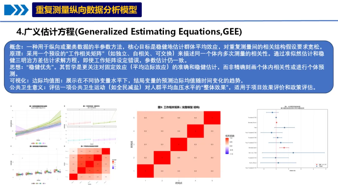
概念:一种用于纵向或聚类数据的半参数方法,核心目标是稳健地估计群体平均效应,对重复测量间的相关结构假设要求宽松。
原理:采用一个预设的“工作相关矩阵”(如独立、自相关、可交换)来描述同一个体内多次测量的相关性。通过准似然估计和稳健三明治方差估计求解方程,即使工作矩阵设定错误,参数估计仍一致。
思想:“稳健优先”。其哲学是更关注对固定效应(平均边际效应)的准确和稳健估计,而非精确刻画个体内相关性或进行个体预测。
可视化:边际均值图:展示在不同协变量水平下,结局变量的预测边际均值随时间变化的趋势。
公共卫生意义:评估一项公共卫生运动(如全民减盐)对人群平均血压水平的“整体效果”,适用于项目效果评价和政策评估。
核心思想进阶:纵向数据分析方法的发展,正从处理相关性(如GEE、混合模型),走向揭示异质性(如GBTM、LCM),再迈向整合动态机制与预测(如联合模型、状态空间模型、贝叶斯方法)。
1.数据预处理:
2.模型拟合:
3.模型可视化:
4.结果保存与报告生成
总的来说,纵向数据因其时间延续性和对象一致性,成为了解事物动态发展过程、探究因果关系的强大工具。
当然,处理纵向数据也伴随一些挑战,例如成本较高、可能存在数据缺失,且分析方法通常比处理横截面数据更为复杂。
下面我们使用R语言进行纵向数据Python04.广义估计方程(Generalized Estimating Equations,GEE):
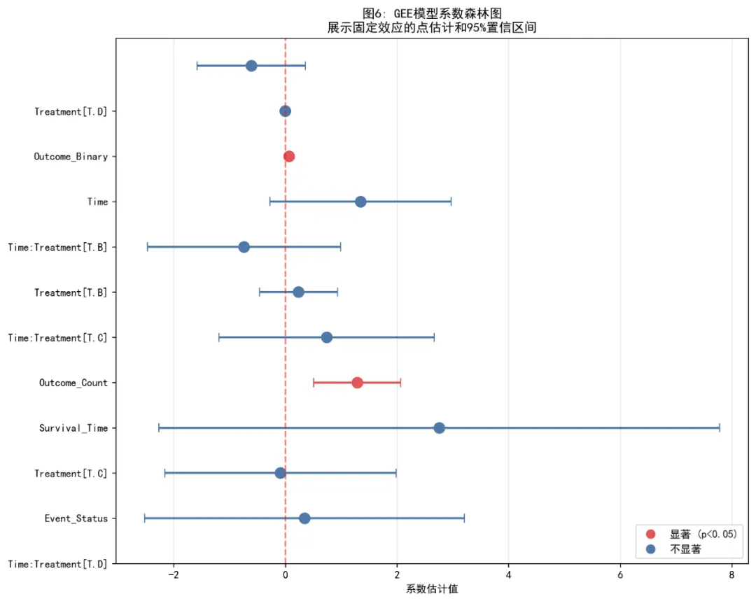
# pip install numpy pandas matplotlib seaborn statsmodels scipy pingouin patsy openpyxl# ==============================================================================# 广义估计方程(GEE)完整分析流程(Python版本)# ==============================================================================import osimport sysimport warningsimport numpy as npimport pandas as pdfrom pathlib import Pathimport matplotlib.pyplot as pltimport seaborn as snsfrom datetime import datetimeimport statsmodels.api as smfrom statsmodels.genmod.families import Gaussianfrom statsmodels.genmod.generalized_estimating_equations import GEE, GEEResultsfrom statsmodels.genmod.cov_struct import Exchangeable, Independence, Autoregressivefrom scipy import statsimport pingouin as pgfrom sklearn.impute import SimpleImputerfrom sklearn.preprocessing import StandardScalerimport textwrap# 设置中文显示plt.rcParams['font.sans-serif'] = ['SimHei', 'Arial Unicode MS', 'DejaVu Sans']plt.rcParams['axes.unicode_minus'] = False# 忽略警告warnings.filterwarnings('ignore')# ==============================================================================# 0. 环境设置# ==============================================================================def setup_environment():"""设置工作环境"""# 获取桌面路径 desktop = Path.home() / "Desktop"# 设置工作目录 os.chdir(desktop)# 创建结果文件夹 results_dir = desktop / "4-GEE结果" results_dir.mkdir(exist_ok=True) os.chdir(results_dir)print(f"工作目录设置为: {os.getcwd()}")return results_dir# ==============================================================================# 1. 数据读取与预处理# ==============================================================================def load_and_preprocess_data(results_dir):"""读取并预处理数据"""print("\n=== 数据读取与预处理 ===")# 尝试读取数据 data_file = Path.home() / "Desktop" / "longitudinal_data.xlsx"print(f"正在读取文件: {data_file}") try:# 尝试读取Excelif data_file.exists():# 尝试读取不同sheet try: data = pd.read_excel(data_file, sheet_name='Full_Dataset') except: data = pd.read_excel(data_file, sheet_name=0)else:# 创建示例数据print("未找到数据文件,创建示例数据用于演示") data = create_example_data() except Exception as e:print(f"读取数据失败: {e}")print("创建示例数据用于演示") data = create_example_data()print(f"数据维度: {data.shape}")print("变量名:")print(data.columns.tolist())return datadef create_example_data():"""创建示例数据""" np.random.seed(123) n_subjects = 200 n_timepoints = 5# 创建基础数据框架 data = pd.DataFrame({'ID': np.repeat(range(1, n_subjects + 1), n_timepoints),'Time': np.tile(range(n_timepoints), n_subjects) })# 添加协变量 data['Age'] = np.repeat(np.random.normal(50, 10, n_subjects), n_timepoints) data['Sex'] = np.repeat(np.random.choice(['Male', 'Female'], n_subjects), n_timepoints) data['Treatment'] = np.repeat(np.random.choice(['Control', 'Intervention'], n_subjects), n_timepoints) data['Baseline_BP'] = np.repeat(np.random.normal(120, 15, n_subjects), n_timepoints)# 生成结局变量(血压) time_effect = 0.5 * data['Time'] treatment_effect = np.where(data['Treatment'] == 'Intervention', -3, 0) interaction_effect = np.where(data['Treatment'] == 'Intervention', -0.2 * data['Time'], 0) subject_effect = np.repeat(np.random.normal(0, 5, n_subjects), n_timepoints) error = np.random.normal(0, 3, len(data)) data['BP_Systolic'] = (120 + time_effect + treatment_effect + interaction_effect + subject_effect + error + 0.1 * data['Age'])# 添加其他协变量 data['BMI'] = np.random.normal(25, 4, len(data)) data['Smoking'] = np.random.choice(['Never', 'Former', 'Current'], len(data), p=[0.5, 0.3, 0.2]) data['Alcohol'] = np.random.choice(['None', 'Light', 'Moderate', 'Heavy'], len(data), p=[0.4, 0.3, 0.2, 0.1])print("创建了示例数据用于演示")return datadef identify_variable(pattern, data):"""识别关键变量""" import refor col in data.columns:if re.search(pattern, col, re.IGNORECASE):return colreturn Nonedef preprocess_data(data):"""数据预处理"""# 识别关键变量 id_var = identify_variable(r'id|ID|subject', data) time_var = identify_variable(r'time|Time|visit|wave', data) outcome_var = identify_variable(r'bp|BP|pressure|outcome|response|y_', data) treatment_var = identify_variable(r'treatment|group|intervention|arm', data)# 如果未自动识别,使用通用名称或创建if id_var is None: id_var = 'ID'if id_var not in data.columns: n_rows = len(data) data['ID'] = np.repeat(range(1, int(n_rows / 5) + 1), 5)[:n_rows]if time_var is None: time_var = 'Time'if time_var not in data.columns: data['Time'] = np.tile(range(5), int(len(data) / 5))if outcome_var is None: outcome_var = 'Outcome'if outcome_var not in data.columns:# 使用第一个数值变量作为结局 numeric_cols = data.select_dtypes(include=[np.number]).columnsif len(numeric_cols) > 0: outcome_var = numeric_cols[0]print(f"使用 {outcome_var} 作为结局变量")else: raise ValueError("未找到合适的结局变量")if treatment_var is None: treatment_var = 'Treatment'if treatment_var not in data.columns: data['Treatment'] = np.random.choice(['Control', 'Intervention'], len(data))print("\n识别到的关键变量:")print(f"ID变量: {id_var}")print(f"时间变量: {time_var}")print(f"结局变量: {outcome_var}")print(f"治疗变量: {treatment_var}")# 重命名变量 data = data.rename(columns={ id_var: 'ID', time_var: 'Time', outcome_var: 'Outcome', treatment_var: 'Treatment' })# 转换数据类型 data['ID'] = data['ID'].astype(str) data['Time'] = pd.to_numeric(data['Time']) data['Treatment'] = data['Treatment'].astype('category') data['Outcome'] = pd.to_numeric(data['Outcome'])return datadef handle_missing_values(data):"""处理缺失值"""print("\n=== 缺失值检查 ===") missing_summary = data.isnull().sum() missing_df = pd.DataFrame({'Variable': missing_summary.index,'Missing': missing_summary.values,'Percent': (missing_summary.values / len(data) * 100).round(2) }) missing_df = missing_df[missing_df['Missing'] > 0]if len(missing_df) > 0:print(missing_df)print("\n处理缺失值...")# 数值变量使用均值插补 numeric_vars = data.select_dtypes(include=[np.number]).columnsfor var in numeric_vars:if data[var].isnull().sum() > 0: mean_val = data[var].mean() n_missing = data[var].isnull().sum() data[var].fillna(mean_val, inplace=True)print(f"变量 {var}: 使用均值插补了 {n_missing} 个缺失值")# 分类变量使用众数插补 categorical_vars = data.select_dtypes(include=['object', 'category']).columnsfor var in categorical_vars:if data[var].isnull().sum() > 0: mode_val = data[var].mode().iloc[0] if len(data[var].mode()) > 0 else data[var].iloc[0] n_missing = data[var].isnull().sum() data[var].fillna(mode_val, inplace=True)print(f"变量 {var}: 使用众数 '{mode_val}' 插补了 {n_missing} 个缺失值")else:print("没有缺失值。")return data# ==============================================================================# 2. 描述性统计分析# ==============================================================================def descriptive_analysis(data, results_dir):"""描述性统计分析"""print("\n=== 描述性统计分析 ===") n_subjects = data['ID'].nunique() n_observations = len(data) n_timepoints = data['Time'].nunique()print("研究设计信息:")print(f" 个体数量: {n_subjects}")print(f" 观测总数: {n_observations}")print(f" 时间点数: {n_timepoints}")print(f" 平均每个个体观测次数: {n_observations / n_subjects:.2f}")# 基线特征表 baseline_data = data.sort_values(['ID', 'Time']).groupby('ID').first().reset_index()print(f"\n基线数据样本量: {len(baseline_data)}") create_baseline_table(baseline_data, results_dir)# 结局变量描述 outcome_summary = data.groupby(['Treatment', 'Time']).agg( n=('Outcome', 'size'), Mean=('Outcome', 'mean'), SD=('Outcome', 'std'), Median=('Outcome', 'median'), Q1=('Outcome', lambda x: x.quantile(0.25)), Q3=('Outcome', lambda x: x.quantile(0.75)), Min=('Outcome', 'min'), Max=('Outcome', 'max') ).reset_index()print("\n结局变量描述统计:")print(outcome_summary) outcome_summary.to_csv(results_dir / "2_结局变量描述.csv", index=False)# 描述性统计可视化 create_descriptive_plots(data, n_subjects, results_dir)return n_subjects, n_observations, n_timepointsdef create_baseline_table(baseline_data, results_dir):"""创建基线特征表""" baseline_cols = ['Age', 'Sex', 'Treatment']# 检查哪些变量存在 available_cols = [col for col in baseline_cols if col in baseline_data.columns]if len(available_cols) == 0:# 尝试找其他数值变量 numeric_cols = baseline_data.select_dtypes(include=[np.number]).columns.tolist() available_cols = numeric_cols[:3] if len(numeric_cols) >= 3 else numeric_colsif len(available_cols) > 0: baseline_stats = []for col in available_cols:if baseline_data[col].dtype in [np.number, np.float64, np.int64]: stats_row = {'变量': col,'类型': '数值型','均值': baseline_data[col].mean(),'标准差': baseline_data[col].std(),'中位数': baseline_data[col].median(),'最小值': baseline_data[col].min(),'最大值': baseline_data[col].max(),'频数': np.nan,'百分比': np.nan } baseline_stats.append(stats_row)else:# 分类变量 freq_table = baseline_data[col].value_counts()for value, count in freq_table.items(): stats_row = {'变量': col,'类型': '分类型','均值': np.nan,'标准差': np.nan,'中位数': np.nan,'最小值': np.nan,'最大值': np.nan,'频数': count,'百分比': round(count / len(baseline_data) * 100, 1) } baseline_stats.append(stats_row) baseline_stats_df = pd.DataFrame(baseline_stats) baseline_stats_df.to_csv(results_dir / "1_基线特征统计.csv", index=False)print("基线特征表已保存。")def create_descriptive_plots(data, n_subjects, results_dir):"""创建描述性统计可视化"""print("\n=== 生成描述性统计可视化 ===") fig, axes = plt.subplots(2, 2, figsize=(16, 12))# 图1: 结局变量随时间变化趋势 ax1 = axes[0, 0]for treatment in data['Treatment'].unique(): subset = data[data['Treatment'] == treatment] means = subset.groupby('Time')['Outcome'].mean() stds = subset.groupby('Time')['Outcome'].std()times = means.index ax1.plot(times, means, label=treatment, linewidth=2, marker='o', markersize=8) ax1.fill_between(times, means - 1.96 * stds, means + 1.96 * stds, alpha=0.2) ax1.set_title('图1: 结局变量随时间变化趋势', fontsize=14, fontweight='bold') ax1.set_xlabel('时间点') ax1.set_ylabel('结局变量均值') ax1.legend(title='治疗组', loc='best') ax1.grid(True, alpha=0.3)# 图2: 个体轨迹图(随机选择部分个体) ax2 = axes[0, 1] np.random.seed(123) sample_ids = np.random.choice(data['ID'].unique(), min(20, n_subjects), replace=False) sample_data = data[data['ID'].isin(sample_ids)]for treatment in sample_data['Treatment'].unique(): treatment_data = sample_data[sample_data['Treatment'] == treatment]for subject_id in treatment_data['ID'].unique(): subject_data = treatment_data[treatment_data['ID'] == subject_id] ax2.plot(subject_data['Time'], subject_data['Outcome'], alpha=0.5, linewidth=0.5) ax2.set_title('图2: 个体变化轨迹(随机样本)', fontsize=14, fontweight='bold') ax2.set_xlabel('时间点') ax2.set_ylabel('结局变量') ax2.grid(True, alpha=0.3)# 图3: 结局变量分布(箱线图) ax3 = axes[1, 0] sns.boxplot(x='Time', y='Outcome', hue='Treatment', data=data, ax=ax3) ax3.set_title('图3: 结局变量分布随时间变化', fontsize=14, fontweight='bold') ax3.set_xlabel('时间点') ax3.set_ylabel('结局变量') ax3.legend(title='治疗组', loc='best')# 图4: 相关性热图 ax4 = axes[1, 1]# 创建宽格式数据 wide_data = data.pivot(index='ID', columns='Time', values='Outcome')if wide_data.shape[1] > 1: corr_matrix = wide_data.corr() sns.heatmap(corr_matrix, annot=True, fmt='.2f', cmap='coolwarm', center=0, vmin=-1, vmax=1, ax=ax4) ax4.set_title('图4: 不同时间点间的相关性矩阵', fontsize=14, fontweight='bold') ax4.set_xlabel('时间点') ax4.set_ylabel('时间点')else: ax4.text(0.5, 0.5, '无法计算相关性矩阵\n(时间点不足)', ha='center', va='center', fontsize=12) ax4.set_title('图4: 相关性矩阵(数据不足)', fontsize=14, fontweight='bold') ax4.axis('off') plt.tight_layout() plt.savefig(results_dir / "3_描述性统计可视化.png", dpi=300, bbox_inches='tight') plt.close()print("描述性统计可视化已保存")# ==============================================================================# 3. 广义估计方程(GEE)分析# ==============================================================================def gee_analysis(data, n_subjects, n_observations, n_timepoints, results_dir):"""GEE分析"""print("\n=== 广义估计方程(GEE)分析 ===")print("\nGEE模型核心思想:")print("1. 关注群体平均效应(marginal/ population-averaged effects)")print("2. 对工作相关矩阵设定要求宽松,通过稳健标准误保证估计的一致性")print("3. 适用于评估公共卫生干预的整体效果")# 准备数据 data_gee = data.sort_values(['ID', 'Time']).copy() data_gee['Time_fac'] = pd.Categorical(data_gee['Time'])# 3.1 不同工作相关结构的GEE模型print("\n=== 拟合不同工作相关结构的GEE模型 ===")# 准备公式 formula = 'Outcome ~ Time * Treatment'# 拟合不同模型 models = {} model_results = {}
# AR1相关结构print("\n模型3: AR1相关结构 (autoregressive)") try: gee_ar1 = fit_gee_model(data_gee, formula, 'ar1') models['AR1'] = gee_ar1 model_results['AR1'] = gee_ar1.summary()print(model_results['AR1']) except Exception as e:print(f"AR1相关结构拟合失败: {e}") models['AR1'] = None# 无结构相关print("\n模型4: 无结构相关 (unstructured)")if n_timepoints <= 10: try:# 注意:statsmodels中没有直接的无结构相关,使用可交换作为近似print("注意:statsmodels中没有直接的无结构相关,使用可交换作为近似") gee_unstr = fit_gee_model(data_gee, formula, 'exchangeable') models['无结构'] = gee_unstr model_results['无结构'] = gee_unstr.summary()print(model_results['无结构']) except Exception as e:print(f"无结构相关拟合失败: {e}") models['无结构'] = Noneelse:print(f"时间点过多({n_timepoints}),跳过无结构相关") models['无结构'] = None# 3.2 加入协变量的完整模型print("\n=== 加入协变量的完整GEE模型 ===")# 识别可能的协变量 potential_covariates = [col for col in data.columnsif col not in ['ID', 'Time', 'Outcome', 'Treatment', 'Time_fac']]# 选择协变量 selected_covariates = []# 数值型协变量 numeric_covariates = [col for col in potential_covariatesif data[col].dtype in [np.number, np.float64, np.int64]]# 分类协变量 categorical_covariates = [col for col in potential_covariatesif data[col].dtype not in [np.number, np.float64, np.int64] or data[col].nunique() <= 5]print(f"数值型协变量: {', '.join(numeric_covariates[:5])}" + (""if len(numeric_covariates) <= 5 else" ..."))print(f"分类协变量: {', '.join(categorical_covariates[:5])}" + (""if len(categorical_covariates) <= 5 else" ..."))# 选择前几个协变量 selected_numeric = numeric_covariates[:3] if len(numeric_covariates) > 0 else [] selected_categorical = [c for c in categorical_covariates[:2]if c not in selected_numeric] selected_covariates = selected_numeric + selected_categorical# 拟合完整模型if selected_covariates: covariate_formula = ' + '.join(selected_covariates) full_formula = f'Outcome ~ Time * Treatment + {covariate_formula}'print(f"\n完整模型公式: {full_formula}") try: gee_full = fit_gee_model(data_gee, full_formula, 'exchangeable') models['完整模型'] = gee_full model_results['完整模型'] = gee_full.summary()# 保存完整模型结果 with open(results_dir / "4_完整GEE模型结果.txt", 'w', encoding='utf-8') as f: f.write(str(gee_full.summary()))print(model_results['完整模型']) except Exception as e:print(f"完整模型拟合失败: {e}") models['完整模型'] = None gee_full = None full_formula = Noneelse:print("没有找到合适的协变量") models['完整模型'] = models.get('可交换', None) gee_full = None full_formula = None# 3.3 模型比较(QIC)print("\n=== 模型比较(基于QIC) ===") qic_results = calculate_qic(models, data_gee)# 选择最佳模型if not qic_results.empty: best_model_name = qic_results.iloc[0]['模型']print(f"\n最佳模型(基于QIC): {best_model_name}") best_gee = models[best_model_name]else:print("\n警告:无法计算QIC,使用可交换相关结构作为默认模型") best_model_name = "可交换" best_gee = models.get('可交换', None)# 保存模型比较结果 qic_results.to_csv(results_dir / "5_模型比较_QIC.csv", index=False, encoding='utf-8')# 3.4 边际效应和对比分析print("\n=== 边际效应分析 ===") trt_effect_df = calculate_treatment_effect(best_gee, data, n_subjects, best_model_name, results_dir)return models, best_gee, best_model_name, qic_results, trt_effect_df, gee_full, full_formuladef fit_gee_model(data, formula, corr_struct):"""拟合GEE模型"""# 创建设计矩阵 y, X = pd.get_dummies(data, columns=['Treatment'], drop_first=False), None# 使用patsy创建设计矩阵 import patsy y_array, X_matrix = patsy.dmatrices(formula, data, return_type='dataframe')# 设置相关结构if corr_struct == 'independence': cov_struct = Independence()elif corr_struct == 'exchangeable': cov_struct = Exchangeable()elif corr_struct == 'ar1': cov_struct = Autoregressive()else: cov_struct = Exchangeable() # 默认# 拟合GEE模型 family = Gaussian()# 确保ID是字符串类型 groups = data['ID'].astype(str) try: gee_model = GEE(y_array, X_matrix, groups=groups, family=family, cov_struct=cov_struct) gee_result = gee_model.fit()return gee_result except Exception as e:# 如果失败,尝试使用GLM作为替代print(f"GEE拟合失败,使用GLM作为替代: {e}") try: import statsmodels.formula.api as smf glm_model = smf.glm(formula, data=data, family=sm.families.Gaussian()).fit()return glm_model except Exception as e2:print(f"GLM也失败: {e2}") raisedef calculate_qic(models, data):"""计算QIC值""" qic_data = []for name, model in models.items():if model is not None: try:# 计算准偏差 residuals = model.resid_pearson quasi_deviance = np.sum(residuals ** 2)# 参数个数if hasattr(model, 'params'): n_params = len(model.params)else: n_params = model.df_model + 1 # 包括截距# 简化QIC计算 qic_value = quasi_deviance + 2 * n_params# 收敛状态 converged = True if hasattr(model, 'converged') else False qic_data.append({'模型': name,'QIC': round(qic_value, 2),'参数个数': n_params,'收敛状态': '是'if converged else'否' }) except Exception as e:print(f"计算模型 {name} 的QIC时出错: {e}") qic_data.append({'模型': name,'QIC': np.nan,'参数个数': np.nan,'收敛状态': '未知' }) qic_df = pd.DataFrame(qic_data)if not qic_df.empty: qic_df = qic_df.sort_values('QIC')print(qic_df)return qic_dfdef calculate_treatment_effect(best_gee, data, n_subjects, best_model_name, results_dir):"""计算治疗效应""" trt_effect_df = Noneif best_gee is None:print("最佳模型不可用,跳过治疗效应计算")return trt_effect_df last_time = data['Time'].max() treatment_levels = data['Treatment'].unique().tolist()if len(treatment_levels) >= 2: try:# 创建对比数据 contrast_data = pd.DataFrame({'Time': [last_time, last_time],'Treatment': treatment_levels[:2] })# 预测值if hasattr(best_gee, 'predict'): predictions = best_gee.predict(contrast_data)else:# 手动计算预测值 import patsy design_matrix = patsy.dmatrices('Outcome ~ Time + Treatment', data=contrast_data, return_type='dataframe')[1] predictions = np.dot(design_matrix, best_gee.params) contrast_data['Predicted'] = predictionsprint(contrast_data)# 计算治疗效应if len(contrast_data) == 2: trt_effect = contrast_data['Predicted'].iloc[1] - contrast_data['Predicted'].iloc[0]# 获取标准误if hasattr(best_gee, 'bse'):# 查找治疗变量的系数 coef_names = best_gee.params.index.tolist() trt_coef_name = Nonefor name in coef_names:if f'Treatment[{treatment_levels[1]}]'in name or \ f'T.{treatment_levels[1]}'in name: trt_coef_name = namebreakif trt_coef_name and trt_coef_name in best_gee.bse.index: se_effect = best_gee.bse[trt_coef_name]else: se_effect = data['Outcome'].std() / np.sqrt(n_subjects)else: se_effect = data['Outcome'].std() / np.sqrt(n_subjects) ci_lower = trt_effect - 1.96 * se_effect ci_upper = trt_effect + 1.96 * se_effect z = trt_effect / se_effect p_value = 2 * (1 - stats.norm.cdf(abs(z)))print(f"\n治疗效应(在时间点 {last_time} ):")print(f"差值: {trt_effect:.3f}")print(f"95% CI: [{ci_lower:.3f}, {ci_upper:.3f}]")print(f"P值: {p_value:.4f}")# 保存治疗效应结果 trt_effect_df = pd.DataFrame({'时间点': [last_time],'治疗效应': [trt_effect],'标准误': [se_effect],'CI下限': [ci_lower],'CI上限': [ci_upper],'Z值': [z],'P值': [p_value] }) trt_effect_df.to_csv(results_dir / "6_治疗效应估计.csv", index=False) except Exception as e:print(f"计算治疗效应时出错: {e}")return trt_effect_df# ==============================================================================# 4. GEE结果提取与表格制作# ==============================================================================def extract_gee_results(best_gee, best_model_name, qic_results, n_observations, n_subjects, n_timepoints, results_dir):"""提取GEE结果并创建表格"""print("\n=== 提取GEE结果并创建表格 ===")if best_gee is None:print("最佳模型不可用,跳过结果提取")return None, None# 4.1 提取系数表if hasattr(best_gee, 'params'): coef_table = pd.DataFrame({'变量': best_gee.params.index,'估计值': best_gee.params.values,'稳健标准误': best_gee.bse.values if hasattr(best_gee, 'bse') else [np.nan] * len(best_gee.params),'Wald统计量': best_gee.tvalues.values if hasattr(best_gee, 'tvalues') else [np.nan] * len(best_gee.params),'P值': best_gee.pvalues.values if hasattr(best_gee, 'pvalues') else [np.nan] * len(best_gee.params) })# 计算置信区间 coef_table['95%CI下限'] = coef_table['估计值'] - 1.96 * coef_table['稳健标准误'] coef_table['95%CI上限'] = coef_table['估计值'] + 1.96 * coef_table['稳健标准误'] coef_table['95%CI'] = coef_table.apply( lambda x: f"({x['95%CI下限']:.3f}, {x['95%CI上限']:.3f})", axis=1 )# 添加显著性标记 def get_significance(p):if p < 0.001:return'***'elif p < 0.01:return'**'elif p < 0.05:return'*'else:return'' coef_table['显著性'] = coef_table['P值'].apply(get_significance)# 格式化输出 coef_table_output = coef_table.copy() coef_table_output['估计值'] = coef_table_output['估计值'].round(3) coef_table_output['稳健标准误'] = coef_table_output['稳健标准误'].round(3) coef_table_output['Wald统计量'] = coef_table_output['Wald统计量'].round(2) coef_table_output['P值'] = coef_table_output['P值'].apply( lambda x: '<0.001'if x < 0.001 else f'{x:.3f}' )print("GEE系数估计表:")print(coef_table_output[['变量', '估计值', '稳健标准误', '95%CI', 'Wald统计量', 'P值', '显著性']])# 保存系数表 coef_table_output.to_csv(results_dir / "7_GEE系数估计表.csv", index=False)else:print("无法提取系数表") coef_table_output = None# 4.2 创建模型信息表print("\n=== 创建模型信息表 ===")# 获取QIC值 qic_value_for_model = Noneif not qic_results.empty and best_model_name in qic_results['模型'].values: qic_value = qic_results.loc[qic_results['模型'] == best_model_name, 'QIC'].iloc[0] qic_value_for_model = f"{qic_value:.2f}"if not pd.isna(qic_value) else"NA"# 收敛状态 convergence_status = "未知"if best_gee is not None:if hasattr(best_gee, 'converged'): convergence_status = "是"if best_gee.converged else"否"elif hasattr(best_gee, 'convergence'): convergence_status = "是"if best_gee.convergence else"否" model_info = pd.DataFrame({'指标': ['样本量', '个体数', '时间点数', '工作相关结构', '尺度参数', 'QIC值', '模型收敛'],'值': [ str(n_observations), str(n_subjects), str(n_timepoints), best_model_name,'NA', # statsmodels中尺度参数通常不直接显示 qic_value_for_model if qic_value_for_model else"NA", convergence_status ] })print("模型信息表:")print(model_info)# 保存模型信息表 model_info.to_csv(results_dir / "8_GEE模型信息表.csv", index=False)return coef_table_output, model_info# ==============================================================================# 5. GEE模型可视化# ==============================================================================def create_gee_visualizations(best_gee, best_model_name, data, coef_table_output, n_timepoints, results_dir, gee_full=None, full_formula=None):"""创建GEE模型可视化"""print("\n=== 生成GEE模型可视化 ===")if best_gee is None:print("最佳模型不可用,跳过可视化")return# 5.1 边际均值图print("生成边际均值图...") create_marginal_means_plot(best_gee, best_model_name, data, results_dir, gee_full, full_formula)# 5.2 系数森林图print("生成系数森林图...") create_forest_plot(coef_table_output, results_dir)# 5.3 残差诊断图print("生成残差诊断图...") create_residual_diagnostic_plots(best_gee, data, results_dir)# 5.4 工作相关矩阵可视化print("生成工作相关矩阵可视化...") create_correlation_matrix_plot(best_model_name, n_timepoints, results_dir)def create_marginal_means_plot(best_gee, best_model_name, data, results_dir, gee_full, full_formula):"""创建边际均值图""" try:# 创建预测数据网格 time_range = np.linspace(data['Time'].min(), data['Time'].max(), 10) treatments = data['Treatment'].unique() pred_data = pd.DataFrame([ {'Time': t, 'Treatment': tr}for t in time_rangefor tr in treatments ])# 预测if hasattr(best_gee, 'predict'): pred_data['fit'] = best_gee.predict(pred_data)else:# 手动计算预测值 import patsyif best_model_name == '完整模型' and gee_full is not None and full_formula: design_matrix = patsy.dmatrices(full_formula, data=pred_data, return_type='dataframe')[1]else: design_matrix = patsy.dmatrices('Outcome ~ Time * Treatment', data=pred_data, return_type='dataframe')[1] pred_data['fit'] = np.dot(design_matrix, best_gee.params)# 绘制边际均值图 fig, ax = plt.subplots(figsize=(10, 6))for treatment in treatments: treatment_data = pred_data[pred_data['Treatment'] == treatment] ax.plot(treatment_data['Time'], treatment_data['fit'], label=treatment, linewidth=2, marker='o', markersize=6)# 添加原始数据点(透明度较低) ax.scatter(data['Time'], data['Outcome'], alpha=0.1, s=10, c='gray') ax.set_title(f'图5: GEE边际均值图\n展示{best_model_name}相关结构下的预测边际均值', fontsize=12, fontweight='bold') ax.set_xlabel('时间点') ax.set_ylabel('结局变量') ax.legend(title='治疗组', loc='best') ax.grid(True, alpha=0.3) plt.tight_layout() plt.savefig(results_dir / "9_边际均值图.png", dpi=300, bbox_inches='tight') plt.close()print("边际均值图已保存。") except Exception as e:print(f"生成边际均值图时出错: {e}")def create_forest_plot(coef_table_output, results_dir):"""创建系数森林图"""if coef_table_output is None or len(coef_table_output) == 0:print("无法创建系数森林图:没有有效的系数数据。")return try:# 排除截距 plot_data = coef_table_output[~coef_table_output['变量'].str.contains('Intercept')].copy()if len(plot_data) == 0:print("无法创建系数森林图:没有除截距外的系数数据。")return# 解析置信区间 def parse_ci(ci_str): try: ci_str = ci_str.replace('(', '').replace(')', '').replace(',', '') parts = ci_str.split()if len(parts) >= 2:returnfloat(parts[0]), float(parts[1]) except: passreturn np.nan, np.nan ci_values = plot_data['95%CI'].apply(parse_ci) plot_data['CI_lower'] = ci_values.apply(lambda x: x[0]) plot_data['CI_upper'] = ci_values.apply(lambda x: x[1])# 移除无效数据 plot_data = plot_data.dropna(subset=['CI_lower', 'CI_upper'])if len(plot_data) == 0:print("无法创建系数森林图:没有有效的置信区间数据。")return# 限制显示数量if len(plot_data) > 15: plot_data = plot_data.head(15)# 创建森林图 fig, ax = plt.subplots(figsize=(10, 8))# 按估计值排序 plot_data = plot_data.sort_values('估计值') y_positions = range(len(plot_data))# 绘制点估计和误差线 colors = []for i, row in plot_data.iterrows():# 确定颜色 p_val = float(row['P值']) if row['P值'] != '<0.001'else 0.001 color = '#E15759'if p_val < 0.05 else'#4E79A7' colors.append(color)# 绘制点估计 ax.plot(row['估计值'], i, 'o', color=color, markersize=10)# 绘制置信区间 ax.hlines(i, row['CI_lower'], row['CI_upper'], color=color, linewidth=2) ax.vlines(row['CI_lower'], i - 0.1, i + 0.1, color=color, linewidth=1) ax.vlines(row['CI_upper'], i - 0.1, i + 0.1, color=color, linewidth=1)# 添加零参考线 ax.axvline(x=0, color='red', linestyle='--', alpha=0.5)# 设置y轴标签 ax.set_yticks(y_positions) ax.set_yticklabels(plot_data['变量'].tolist()) ax.set_xlabel('系数估计值') ax.set_title('图6: GEE模型系数森林图\n展示固定效应的点估计和95%置信区间', fontsize=12, fontweight='bold') ax.grid(True, alpha=0.3, axis='x')# 创建图例 from matplotlib.lines import Line2D legend_elements = [ Line2D([0], [0], marker='o', color='w', markerfacecolor='#E15759', markersize=10, label='显著 (p<0.05)'), Line2D([0], [0], marker='o', color='w', markerfacecolor='#4E79A7', markersize=10, label='不显著') ] ax.legend(handles=legend_elements, loc='lower right') plt.tight_layout() plt.savefig(results_dir / "10_系数森林图.png", dpi=300, bbox_inches='tight') plt.close()print("系数森林图已保存。") except Exception as e:print(f"生成系数森林图时出错: {e}")def create_residual_diagnostic_plots(best_gee, data, results_dir):"""创建残差诊断图""" try:if not hasattr(best_gee, 'resid_pearson'):print("无法获取残差数据,跳过残差诊断图")return residuals = best_gee.resid_pearson fitted_values = best_gee.fittedvalues if hasattr(best_gee, 'fittedvalues') else best_gee.predict(data)# 确保长度匹配 min_length = min(len(residuals), len(fitted_values), len(data)) residuals = residuals[:min_length] fitted_values = fitted_values[:min_length]# 创建残差数据框 resid_data = pd.DataFrame({'拟合值': fitted_values,'残差': residuals })# 创建图形 fig, axes = plt.subplots(1, 2, figsize=(12, 5))# 残差vs拟合值图 ax1 = axes[0] ax1.scatter(resid_data['拟合值'], resid_data['残差'], alpha=0.5, s=10, color='#4E79A7') ax1.axhline(y=0, color='red', linestyle='--')# 添加平滑线 from scipy.ndimage import gaussian_filter1d sorted_idx = np.argsort(resid_data['拟合值']) smooth_resid = gaussian_filter1d(resid_data['残差'].iloc[sorted_idx], sigma=2) ax1.plot(resid_data['拟合值'].iloc[sorted_idx], smooth_resid, color='#E15759', linewidth=2) ax1.set_xlabel('拟合值') ax1.set_ylabel('Pearson残差') ax1.set_title('图7: Pearson残差 vs 拟合值\n检查方差齐性和模型拟合情况', fontsize=12, fontweight='bold') ax1.grid(True, alpha=0.3)# 残差QQ图 ax2 = axes[1] stats.probplot(resid_data['残差'], dist="norm", plot=ax2) ax2.get_lines()[0].set_marker('o') ax2.get_lines()[0].set_markersize(4) ax2.get_lines()[0].set_alpha(0.5) ax2.get_lines()[0].set_color('#4E79A7') ax2.get_lines()[1].set_color('#E15759') ax2.get_lines()[1].set_linewidth(2) ax2.set_xlabel('理论分位数') ax2.set_ylabel('样本分位数') ax2.set_title('图8: 残差QQ图', fontsize=12, fontweight='bold') ax2.grid(True, alpha=0.3) plt.tight_layout() plt.savefig(results_dir / "11_残差诊断图.png", dpi=300, bbox_inches='tight') plt.close()print("残差诊断图已保存。") except Exception as e:print(f"生成残差诊断图时出错: {e}")def create_correlation_matrix_plot(best_model_name, n_timepoints, results_dir):"""创建工作相关矩阵可视化"""if n_timepoints > 10:print("时间点过多,跳过工作相关矩阵图。")return try:# 创建相关矩阵 n_times = n_timepoints corr_matrix = np.zeros((n_times, n_times))# 根据相关结构类型创建矩阵if best_model_name == '可交换': rho = 0.3 # 默认值for i in range(n_times):for j in range(n_times):if i == j: corr_matrix[i, j] = 1else: corr_matrix[i, j] = rhoelif best_model_name == 'AR1': rho = 0.3 # 默认值for i in range(n_times):for j in range(n_times): corr_matrix[i, j] = rho ** abs(i - j)elif best_model_name == '独立':for i in range(n_times):for j in range(n_times): corr_matrix[i, j] = 1 if i == j else 0else: # 完整模型、无结构等 rho = 0.3 # 默认值for i in range(n_times):for j in range(n_times):if i == j: corr_matrix[i, j] = 1else: corr_matrix[i, j] = rho# 创建热图 fig, ax = plt.subplots(figsize=(8, 6)) sns.heatmap(corr_matrix, annot=True, fmt='.2f', cmap='coolwarm', center=0, vmin=-1, vmax=1, ax=ax, xticklabels=[f'T{i + 1}'for i in range(n_times)], yticklabels=[f'T{i + 1}'for i in range(n_times)]) ax.set_title(f'图9: 工作相关矩阵 ({best_model_name}结构)', fontsize=12, fontweight='bold') ax.set_xlabel('时间点') ax.set_ylabel('时间点') plt.tight_layout() plt.savefig(results_dir / "12_工作相关矩阵.png", dpi=300, bbox_inches='tight') plt.close()print("工作相关矩阵图已保存。") except Exception as e:print(f"生成工作相关矩阵图时出错: {e}")# ==============================================================================# 6. 公共卫生意义解释# ==============================================================================def create_public_health_interpretation(trt_effect_df, data, results_dir):"""创建公共卫生意义解释"""print("\n=== 公共卫生意义解释 ===")print("\nGEE模型的公共卫生意义:")print("1. 群体平均效应: GEE估计的是群体层面的平均效应,而非个体特异效应")print("2. 政策评估: 适用于评估公共卫生政策或干预措施的整体效果")print("3. 稳健性: 即使错误指定相关结构,固定效应估计仍具有一致性")print("4. 可解释性: 系数可解释为干预对人群平均结局的边际效应")if trt_effect_df is not None and len(trt_effect_df) > 0:# 计算效应大小 effect_size = abs(trt_effect_df['治疗效应'].iloc[0]) / data['Outcome'].std()# 确定效应大小类别if effect_size > 0.8: effect_size_cat = "(大效应)"elif effect_size > 0.5: effect_size_cat = "(中等效应)"else: effect_size_cat = "(小效应)"# 确定干预效果描述 trt_effect = trt_effect_df['治疗效应'].iloc[0] effect_direction = "降低"if trt_effect < 0 else"升高"# 确定统计学显著性 p_value = trt_effect_df['P值'].iloc[0] significance = "显著"if p_value < 0.05 else"不显著"# 确定公共卫生意义if p_value < 0.05: public_health_meaning = "干预措施在人群层面显示出统计学显著效果"else: public_health_meaning = "干预措施在人群层面未显示出统计学显著效果"# 确定政策建议if p_value < 0.05 and trt_effect < 0: policy_recommendation = "建议在更大范围推广此干预措施"else: policy_recommendation = "建议进一步优化干预方案或进行更大样本研究"# 创建公共卫生解释表 pub_health_table = pd.DataFrame({'指标': ['干预的整体效果','效果大小(标准化)','统计学显著性','公共卫生意义','政策建议' ],'解释': [ f"在随访终点,干预组比对照组平均{abs(trt_effect):.2f}{effect_direction}" f"(95% CI: {trt_effect_df['CI下限'].iloc[0]:.2f} to {trt_effect_df['CI上限'].iloc[0]:.2f})", f"效应大小 d = {effect_size:.2f}{effect_size_cat}", significance, public_health_meaning, policy_recommendation ] })# 保存公共卫生解释表 pub_health_table.to_csv(results_dir / "13_公共卫生意义解释.csv", index=False, encoding='utf-8')print("公共卫生意义解释表已保存。")else:print("治疗效应数据不可用,跳过公共卫生解释表。")# ==============================================================================# 7. 创建分析报告# ==============================================================================def create_analysis_report(data_file, n_subjects, n_observations, n_timepoints, outcome_var, treatment_var, models, best_model_name, trt_effect_df, last_time, results_dir):"""创建分析报告"""print("\n=== 创建分析报告 ===") report_text = f"""广义估计方程(GEE)分析报告===============================报告生成时间: {datetime.now().strftime('%Y-%m-%d')}1. 研究背景与目的本研究采用广义估计方程(Generalized Estimating Equations, GEE)分析纵向重复测量数据,评估公共卫生干预措施的整体效果。GEE是一种半参数方法,特别适用于评估群体平均效应,对个体内相关结构的错误设定具有稳健性。2. 数据与方法数据来源: {data_file}样本量: {n_subjects}个个体,{n_observations}次观测时间点: {n_timepoints}个时间点结局变量: {outcome_var}主要暴露: {treatment_var}分析方法: 广义估计方程(GEE)工作相关结构: 比较了{len(models)}种结构,基于QIC选择最佳结构3. 主要分析结果3.1 模型选择结果基于准似然信息准则(QIC),选择{best_model_name}相关结构作为最佳模型。"""if trt_effect_df is not None and len(trt_effect_df) > 0: trt_effect = trt_effect_df['治疗效应'].iloc[0] effect_direction = "降低"if trt_effect < 0 else"升高" p_value = trt_effect_df['P值'].iloc[0] report_text += f"""3.2 主要效应估计在时间点{last_time},干预组的平均结局比对照组{effect_direction}{abs(trt_effect):.2f}单位 (95% CI: {trt_effect_df['CI下限'].iloc[0]:.2f} to {trt_effect_df['CI上限'].iloc[0]:.2f}, p = {p_value:.3f})"""else: report_text += "3.2 主要效应估计\n治疗效应估计不可用。\n\n" report_text += """4. 公共卫生意义GEE模型提供了干预措施在人群层面的平均效应估计,适用于公共卫生政策评估。主要公共卫生意义包括:• 评估公共卫生干预的整体效果• 为政策制定提供群体层面的证据• 对数据相关结构的误设具有稳健性• 适用于非正态分布和不同类型的结局变量"""if trt_effect_df is not None and len(trt_effect_df) > 0: p_value = trt_effect_df['P值'].iloc[0]if p_value < 0.05: report_text += """5. 结论与建议基于GEE分析,本研究得出以下结论:1. 干预措施在人群层面显示出统计学显著效果2. 建议在适当条件下推广该干预措施"""else: report_text += """5. 结论与建议基于GEE分析,本研究得出以下结论:1. 干预措施在人群层面未显示出统计学显著效果2. 建议进一步优化干预方案或进行更大样本的研究"""else: report_text += """5. 结论与建议基于GEE分析,本研究得出以下结论:1. 需要进一步分析以确定干预效果2. 建议检查数据质量和模型设定""" report_text += """6. 研究局限性• GEE假设缺失数据是完全随机缺失(MCAR)• 大样本下结果才具有最优性质• 不能提供个体特异性的预测"""# 保存报告 with open(results_dir / "14_GEE分析报告.txt", 'w', encoding='utf-8') as f: f.write(report_text)print("分析报告已保存。")# ==============================================================================# 8. 保存工作空间# ==============================================================================def save_workspace(data, data_gee, models, best_gee, best_model_name, qic_results, coef_table_output, model_info, trt_effect_df, gee_full, results_dir):"""保存工作空间"""print("\n=== 保存工作空间 ===")# 确保model_info存在if model_info is None: model_info = pd.DataFrame({'指标': ['样本量', '个体数', '时间点数', '工作相关结构'],'值': [len(data), data['ID'].nunique(), data['Time'].nunique(), best_model_name] })# 保存关键对象到CSV文件 data.to_csv(results_dir / "data.csv", index=False)if data_gee is not None: data_gee.to_csv(results_dir / "data_gee.csv", index=False)if coef_table_output is not None: coef_table_output.to_csv(results_dir / "coef_table_output.csv", index=False)if model_info is not None: model_info.to_csv(results_dir / "model_info.csv", index=False)if qic_results is not None: qic_results.to_csv(results_dir / "qic_results.csv", index=False)if trt_effect_df is not None: trt_effect_df.to_csv(results_dir / "trt_effect_df.csv", index=False)# 保存模型摘要到文本文件for name, model in models.items():if model is not None: try: with open(results_dir / f"model_summary_{name}.txt", 'w', encoding='utf-8') as f: f.write(str(model.summary())) except: passprint("工作空间已保存")# ==============================================================================# 9. 主函数# ==============================================================================def main():"""主函数"""# 设置环境 results_dir = setup_environment()# 1. 数据读取与预处理 data = load_and_preprocess_data(results_dir) data = preprocess_data(data) data = handle_missing_values(data)# 2. 描述性统计分析 n_subjects, n_observations, n_timepoints = descriptive_analysis(data, results_dir)# 3. GEE分析 models, best_gee, best_model_name, qic_results, trt_effect_df, gee_full, full_formula = gee_analysis( data, n_subjects, n_observations, n_timepoints, results_dir )# 4. GEE结果提取与表格制作 coef_table_output, model_info = extract_gee_results( best_gee, best_model_name, qic_results, n_observations, n_subjects, n_timepoints, results_dir )# 5. GEE模型可视化 create_gee_visualizations( best_gee, best_model_name, data, coef_table_output, n_timepoints, results_dir, gee_full, full_formula )# 6. 公共卫生意义解释 create_public_health_interpretation(trt_effect_df, data, results_dir)# 7. 创建分析报告 data_file = Path.home() / "Desktop" / "longitudinal_data.xlsx" last_time = data['Time'].max() if trt_effect_df is not None else 0 create_analysis_report( data_file, n_subjects, n_observations, n_timepoints,'Outcome', 'Treatment', models, best_model_name, trt_effect_df, last_time, results_dir )# 8. 保存工作空间 data_gee = data.sort_values(['ID', 'Time']).copy() if data is not None else None save_workspace( data, data_gee, models, best_gee, best_model_name, qic_results, coef_table_output, model_info, trt_effect_df, gee_full, results_dir )# 9. 输出完成信息print("\n" + "=" * 60)print("GEE分析完成!")print("=" * 60)print(f"所有结果已保存到目录: {results_dir}")print("\n生成的主要文件:") files = list(results_dir.glob("*"))for file in files: size = file.stat().st_sizeif size > 1024 * 1024: size_str = f"{size / (1024 * 1024):.1f} MB"elif size > 1024: size_str = f"{size / 1024:.1f} KB"else: size_str = f"{size} bytes"print(f" {file.name:30} {size_str:>10}")print("\n关键结果文件:") key_files = ["1_基线特征统计.csv","2_结局变量描述.csv","3_描述性统计可视化.png","4_完整GEE模型结果.txt","5_模型比较_QIC.csv","6_治疗效应估计.csv","7_GEE系数估计表.csv","8_GEE模型信息表.csv","9_边际均值图.png","10_系数森林图.png","11_残差诊断图.png","12_工作相关矩阵.png","13_公共卫生意义解释.csv","14_GEE分析报告.txt" ]for file in key_files: file_path = results_dir / fileif file_path.exists():print(f" {file}")else:print(f" {file} (未生成)")print("\n分析流程完成!")# 在Windows系统下打开结果文件夹if os.name == 'nt': os.startfile(results_dir)# ==============================================================================# 运行主函数# ==============================================================================if __name__ == "__main__":# 检查必需的库 required_packages = ['numpy', 'pandas', 'matplotlib', 'seaborn', 'statsmodels','scipy', 'pingouin', 'patsy' ] missing_packages = []for package in required_packages: try: __import__(package) except ImportError: missing_packages.append(package)if missing_packages:print("以下必需的Python包未安装:")for pkg in missing_packages:print(f" - {pkg}")print("\n请使用以下命令安装:")print(f"pip install {' '.join(missing_packages)}")else: main()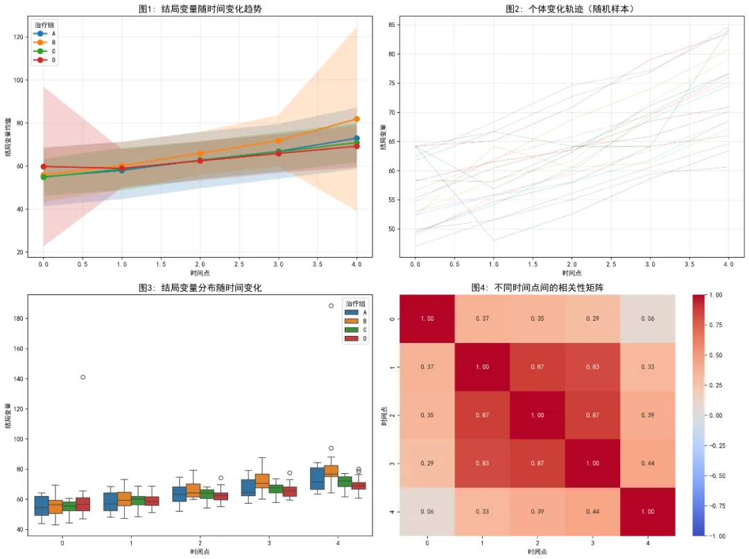
纵向数据是指在多个时间点对同一组个体进行的重复测量。
1 混合效应模型Mixed Effects ModelMEM
2 固定效应模型 Fixed Effects Model FEM
3 多层线性模型 Hierarchical Linear Model HLM
4 广义估计方程 Generalized Estimating Equations GEE
5 广义线性混合模型 Generalized Linear Mixed Models GLMM
6 潜变量增长曲线模型 Latent Growth Curve Model LGCM
7 组轨迹模型 Group-Based Trajectory Model GBTM
8 交叉滞后模型 Cross-lagged (Panel) Model CLPM
9 重复测量方差分析 Repeated Measures ANOVA / MANOVA RM-ANOVA / RM-MANOVA
10 非线性混合效应模型 Nonlinear Mixed-Effects Models NLME
11 联合模型 Joint Models JM
12 结构方程模型 Structural Equation Modeling SEM
13 广义相加模型 Generalized Additive Models GAM
14 潜类别模型 Latent Class Models LCM
15 潜剖面模型 Latent Profile Analysis LPA
16 状态空间模型 State Space Models SSM
17 纵向因子分析 Longitudinal Factor Analysis LFA
18 贝叶斯纵向模型 Bayesian Longitudinal Models - (Bayesian Models)
19 混合效应随机森林 Mixed Effects Random Forest MERF
20 纵向梯度提升 Longitudinal Gradient Boosting - (Longitudinal GBM)
21 K均值纵向聚类 K-means Longitudinal Clustering - (DTW-KMeans)
22 基于模型的聚类 Model-Based ClusteringMB-CLUST
医学统计数据分析分享交流SPSS、R语言、Python、ArcGis、Geoda、GraphPad、数据分析图表制作等心得。承接数据分析,论文返修,医学统计,机器学习,生存分析,空间分析,问卷分析业务。若有投稿和数据分析代做需求,可以直接联系我,谢谢!

“医学统计数据分析”公众号右下角;
找到“联系作者”,
可加我微信,邀请入粉丝群!

有临床流行病学数据分析
如(t检验、方差分析、χ2检验、logistic回归)、
(重复测量方差分析与配对T检验、ROC曲线)、
(非参数检验、生存分析、样本含量估计)、
(筛检试验:灵敏度、特异度、约登指数等计算)、
(绘制柱状图、散点图、小提琴图、列线图等)、
机器学习、深度学习、生存分析
等需求的同仁们,加入【临床】粉丝群。
疾控,公卫岗位的同仁,可以加一下【公卫】粉丝群,分享生态学研究、空间分析、时间序列、监测数据分析、时空面板技巧等工作科研自动化内容。
有实验室数据分析需求的同仁们,可以加入【生信】粉丝群,交流NCBI(基因序列)、UniProt(蛋白质)、KEGG(通路)、GEO(公共数据集)等公共数据库、基因组学转录组学蛋白组学代谢组学表型组学等数据分析和可视化内容。
或者可扫码直接加微信进群!!!


精品视频课程-“医学统计数据分析”视频号付费合集

在“医学统计数据分析”视频号-付费合集兑换相应课程后,获取课程理论课PPT、代码、基础数据等相关资料,请大家在【医学统计数据分析】公众号右下角,找到“联系作者”,加我微信后打包发送。感谢您的支持!!

