期刊图片复现|Python绘制遥感影像空间分布图
- 2026-07-04 05:07:19
期刊图片复现|Python绘制遥感影像空间分布图

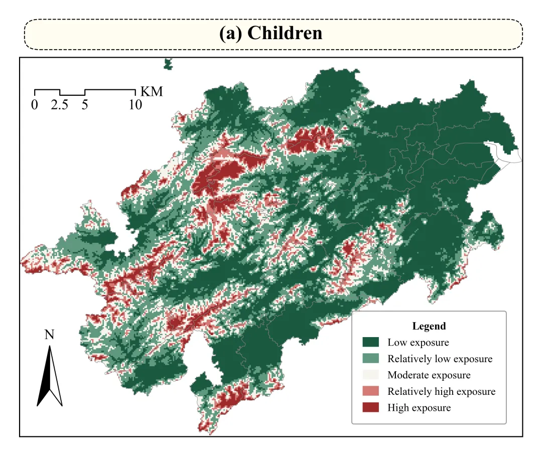
论文:Advancing climate justice for vulnerable groups: Optimizing spatial 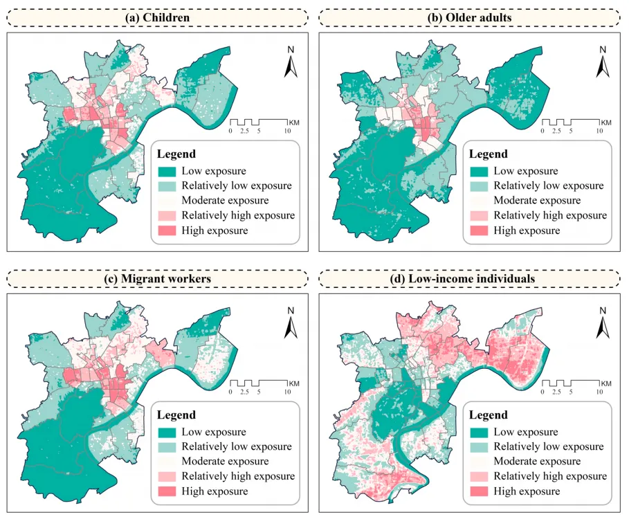
论文原图 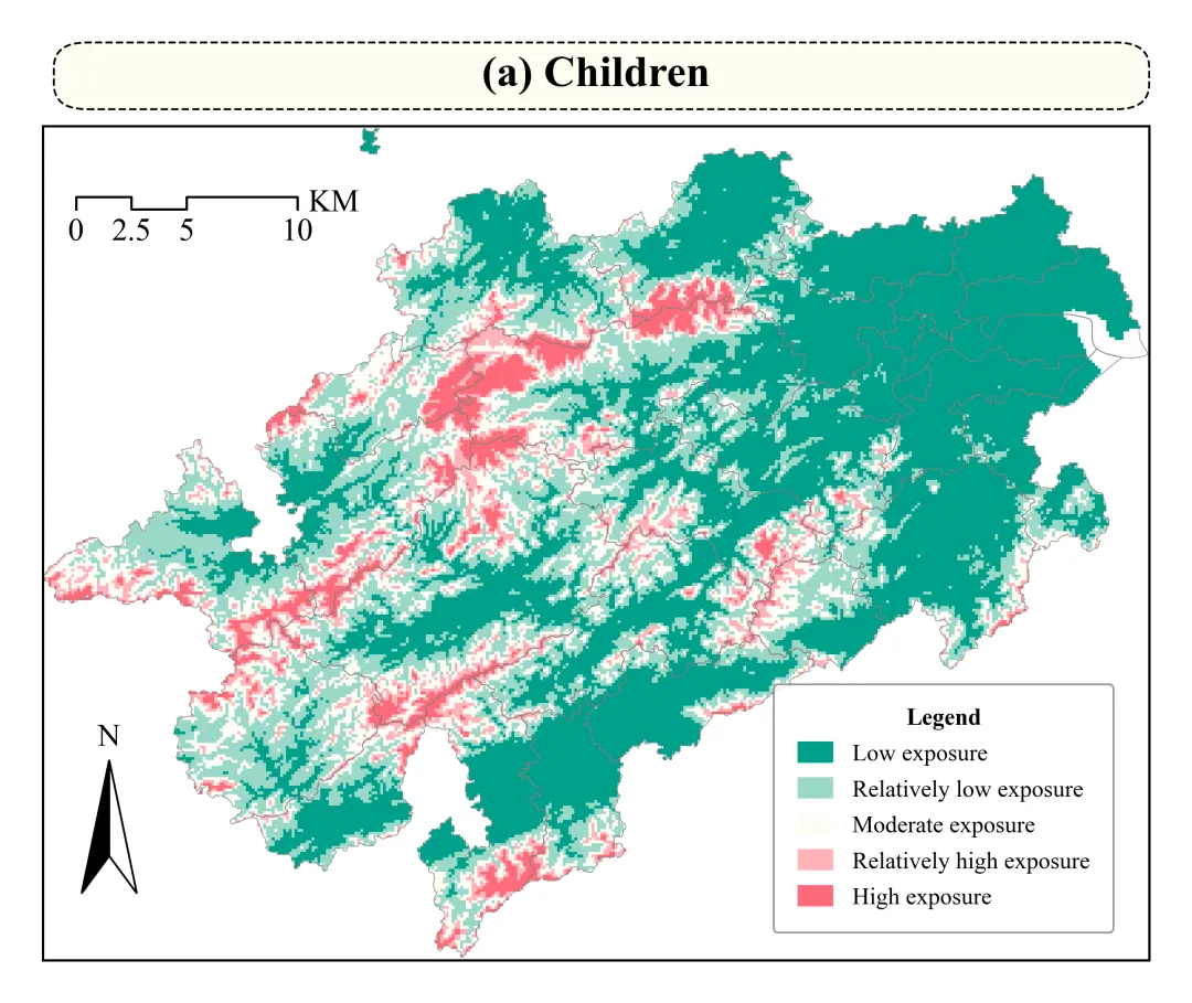
仿图 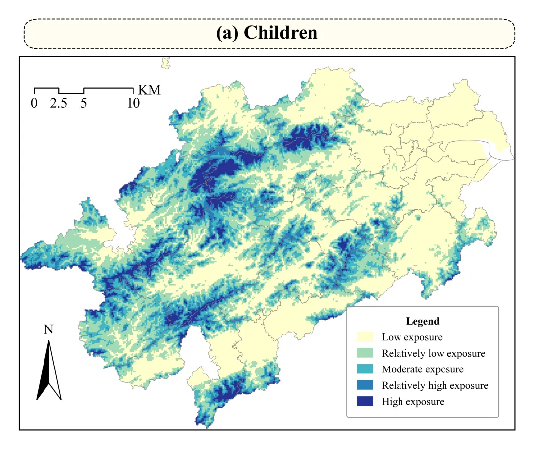
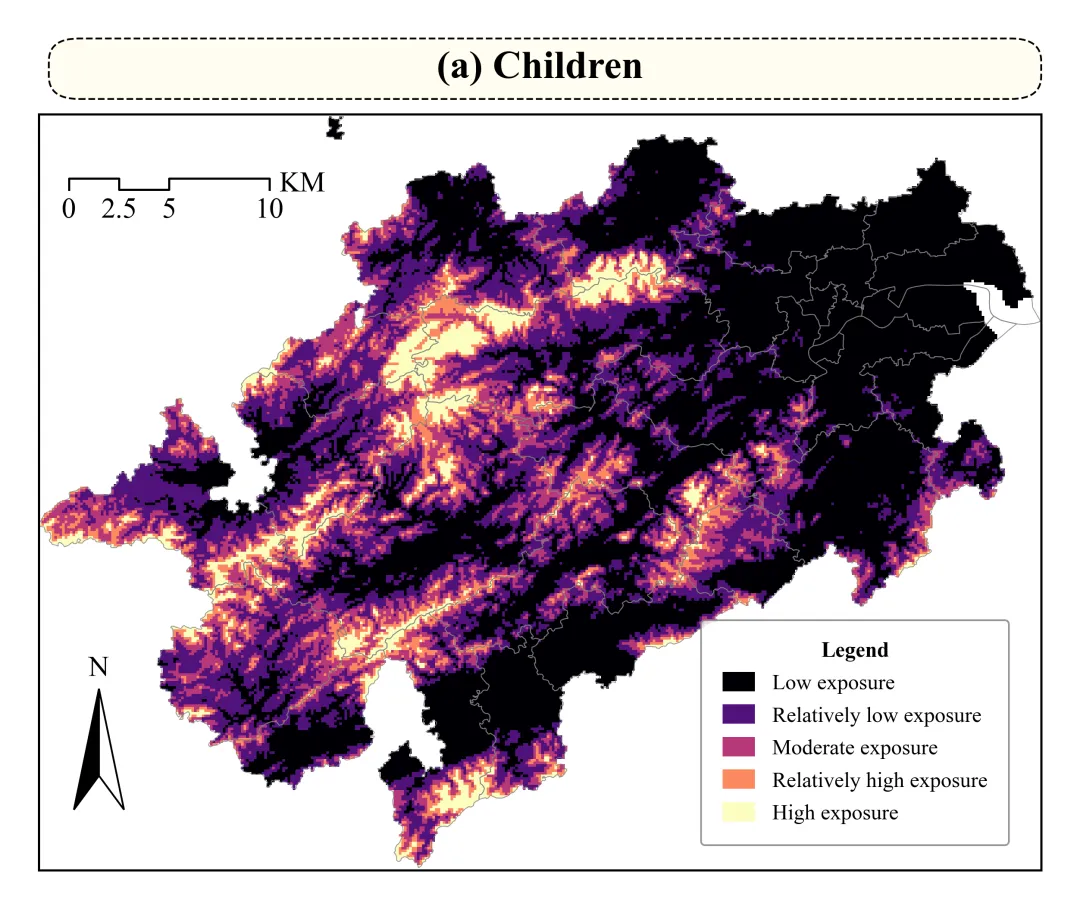
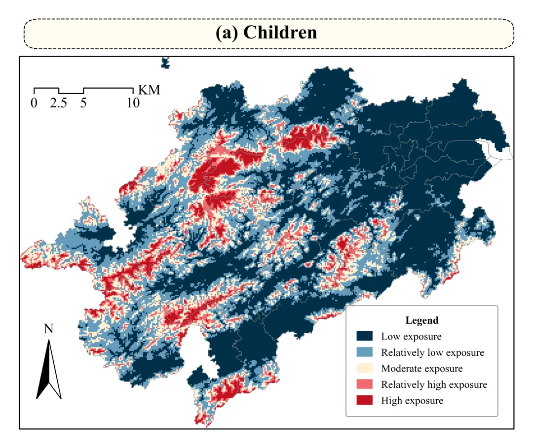
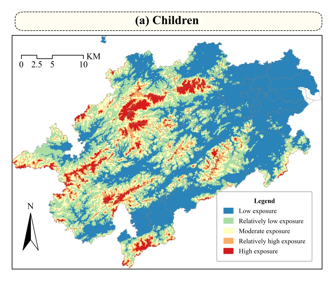
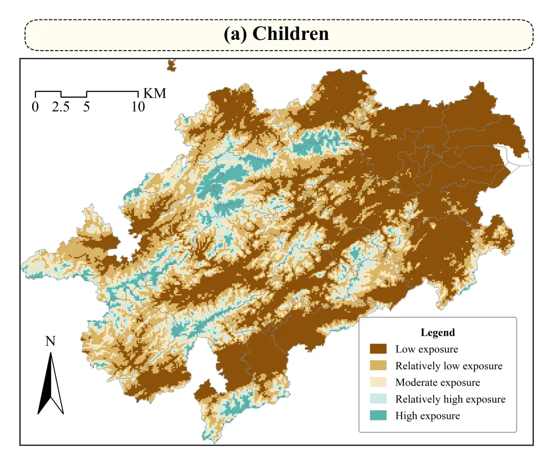
多种配色 


库的导入以及字体设置 

颜色库的设置以及配色方案的选择 

绘图函数:渲染底图与矢量叠加。创建连续渐变色,根据阈值边界将数据切分为5个离散的色块。创建画布。将栅格影像数据画在图上。使用矢量数据绘制出研究区轮廓线条。 

绘图函数:设置坐标轴范围,设置边框刻度线、经纬度,设置边框线。 

绘图函数:标题框设置以及标题的设置 

绘图函数:图例设置 

绘图函数:指北针的绘制 

绘图函数:比例尺绘制 

执行部分 


期刊图片复现|Python绘制二维偏依赖PDP图 期刊复现|python绘制基于SHAP分析和GAM模型拟合的单特征依赖图 期刊图片复现|python绘制带有渐变颜色shap特征重要性组合图(条形图+蜂巢图) 期刊复现|用Python绘制SHAP特征重要性总览图、依赖图、双特征交互效应SHAP图,解锁XGBoost模型的终极奥秘 期刊图片复现|Python绘制shap重要性蜂巢图+单特征依赖图+交互效应强度气泡图+交互效应依赖图(回归+二分类+分类) 

公众号中的所有所有的免费代码都已经下架了,都并入到付费部分里了,付费合集代码和数据的购买通道已经开通,全部合集100元,后续将会持续更新,决定购买请后台私信我,注意只会分享练习数据和代码文件,不会提供答疑服务,代码文件中已经包含了每行代码的完整注释,购买前请确保真的需要!!!
代码绘制成果展示
configuration of urban blue–green infrastructure to mitigate heat risks leveraging explainable machine learning
代码解释
第一部分
# =========================================================================================# ====================================== 1. 环境设置 =======================================# =========================================================================================import matplotlib.pyplot as pltimport matplotlib.colors as mcolorsimport matplotlib.patches as mpatchesimport rasterioimport numpy as np
第二部分
# =========================================================================================# ======================================2.颜色库=======================================# =========================================================================================COLOR_SCHEMES = {1: ['#00A08A', '#9BD8C9', '#FDFDF5', '#FFB3B9', '#FF6B7A'],}SCHEME_ID = 1 #要使用的配色方案hex_colors = COLOR_SCHEMES.get(SCHEME_ID, COLOR_SCHEMES[1]) #提取配色方案
第三部分
# =========================================================================================# ======================================4.绘图函数======================================# =========================================================================================def plot_exposure_map(data, extent, gdf, bounds, title_text):cmap = mcolors.ListedColormap(hex_colors) #创建离散的颜色映射器norm = mcolors.BoundaryNorm(bounds, cmap.N) #基于数据阈值列表创建一个归一化对象,用于将数值映射到相应的离散颜色块#创建画布fig, ax = plt.subplots(figsize=(10, 8), dpi=300)# 在坐标轴上绘制传入的二维栅格数组图像im = ax.imshow(data, #数据cmap=cmap, #颜色映射norm=norm, #颜色归一化规则extent=extent, #空间范围左, 右, 下, 上interpolation='nearest') #使用最近邻插值,保证像素边缘清晰且不改变原有数值#绘制矢量多边形边界gdf.boundary.plot(ax=ax, #坐标轴edgecolor='gray', #边界线颜色linewidth=1, #边界线宽度alpha=1) #边界线透明度
第四部分
ax.set_aspect('equal') #X轴与Y轴的比例设置ax.set_xlim(extent[0], extent[1]) #X轴的显示范围,使其与栅格数据的左右边界对齐ax.set_ylim(extent[2], extent[3]) #Y轴的显示范围,使其与栅格数据的上下边界对齐# 移除X轴的刻度与经纬度标注ax.set_xticks([])ax.set_yticks([])# 设置边框线for spine in ax.spines.values():spine.set_linewidth(1.2)spine.set_color('black')
第五部分
box_width = 0.97 # 标题背景框的相对宽度box_height = 0.06 #标题背景框的相对高度# 创建矩形背景框title_box = mpatches.FancyBboxPatch((0.02, 1.03), #左下角的相对起始坐标box_width, #宽度box_height, #高度boxstyle="round,pad=0.01,rounding_size=0.03", #圆角edgecolor="black", #背景框边线的颜色facecolor="#FFFDF0", #背景框内部的填充颜色linewidth=1, #边界宽度linestyle="--", #边线型transform=ax.transAxes, # 坐标系clip_on=False, #允许该背景框在坐标轴范围外被绘制而不被裁切zorder=10 #层级)
第六部分
#图例文本labels = ['Low exposure', 'Relatively low exposure', 'Moderate exposure', 'Relatively high exposure','High exposure']# 调用并生成图例,传入前面构建好的图例元素列表legend = ax.legend(handles=legend_elements, #图例元素列表loc='lower right', #位置bbox_to_anchor=(0.97, 0.03), #位置title="Legend", #标题fontsize=12, #字体大小title_fontsize=12, #图例标题文字的字体大小labelspacing=0.5, #图例标签之间的垂直间距borderpad=0.6, #图例框边框与内部元素之间的空白内边距handlelength=1.5, #图例色块的长度比例handleheight=1.0, #图例色块的高度比例frameon=True, #外边框edgecolor='gray', #边框线颜色facecolor='white') #图例框内部填充色legend.get_title().set_fontweight('bold') #获取图例标题对象并设置字体为加粗样式
第七部分
nx, ny = 0.06, 0.24 #指北针图形起点的相对X、Y坐标w, h = 0.025, 0.16 #指北针箭头形状的横向半宽和垂直总高度tail_indent = 0.045 #指北针尾部向内凹陷的垂直深度参数left_polygon = np.array([[nx, ny], [nx - w, ny - h], [nx, ny - h + tail_indent]]) #指北针左半侧多边形的3个顶点坐标right_polygon = np.array([[nx, ny], [nx + w, ny - h], [nx, ny - h + tail_indent]]) #指北针右半侧多边形的3个顶点坐标# 定位在指北针顶端的X坐标ax.text(nx, #Xny + 0.01, #Y'N', #文本ha='center', #水平va='bottom', #垂直fontsize=16, #字体大小transform=ax.transAxes, #坐标系zorder=10) #层级
第八部分
target_scale_degrees = 0.5181 #设置目标比例尺公里对应的经度跨度map_real_width_degrees = extent[1] - extent[0] #经度差scale_fraction = target_scale_degrees / map_real_width_degrees #计算50公里比例尺在整幅地图宽度中所占的相对比例scale_x, scale_y = 0.03, 0.9 #设置比例尺左侧起点的X、Y相对坐标#添加比例尺文本ax.text(scale_x, #Xtext_y, #Y'0', #文本ha='center', #水平va='top', #垂fontsize=font_sz, #字体大小transform=ax.transAxes) #坐标系ax.text(scale_x + frac_25, text_y, '12.5', ha='center', va='top', fontsize=font_sz,transform=ax.transAxes)ax.text(scale_x + frac_50, text_y, '25', ha='center', va='top', fontsize=font_sz, transform=ax.transAxes)ax.text(scale_x + frac_100, text_y, '50', ha='center', va='top', fontsize=font_sz,transform=ax.transAxes)ax.text(scale_x + frac_100 + 0.01, scale_y + step_h / 2, 'KM', ha='left', va='center', fontsize=font_sz,transform=ax.transAxes)
第九部分
# =========================================================================================# ======================================4.绘图函数======================================# =========================================================================================if __name__ == "__main__":tif_path = r'2.tif' #栅格数据的路径shp_path = r'州.shp' #矢量数据的路径title_str = "(a) Children" #主标题if gdf.crs != raster_crs: #判断矢量数据的坐标系与栅格的坐标系是否一致gdf = gdf.to_crs(raster_crs) #若不一致,则将矢量重投影转换到和栅格一样的坐标系下以保证正常叠加#调用绘图函数plot_exposure_map(data=data, #栅格数据数组extent=extent, #边界四至范围gdf=gdf, # 矢量边界bounds=bounds, #分级阈值列表title_text=title_str, # 标题)
如何应用到你自己的数据
1.设置配色方案:
SCHEME_ID = 1 #要使用的配色方案2.设置图例的文本:
labels = ['Low exposure', 'Relatively low exposure', 'Moderate exposure', 'Relatively high exposure', 'High exposure']3.设置图例的文本:
labels = ['Low exposure', 'Relatively low exposure', 'Moderate exposure', 'Relatively high exposure', 'High exposure']4.设置绘图结果的保存地址:
plt.savefig( fr'Final{SCHEME_ID}.png', dpi=300, bbox_inches='tight',pad_inches=0.3)5.设置栅格数据的保存路径:
tif_path = r'杭州.tif' #栅格数据的路径6.设置矢量数据的保存路径:
shp_path = r'杭州.shp' #矢量数据的路7.设置主图的标题:
title_str = "(a) Children" #主标题推荐
获取方式
本文来自网友投稿或网络内容,如有侵犯您的权益请联系我们删除,联系邮箱:wyl860211@qq.com 。
随机文章
-
 10个月宝宝每天需要喝多少奶粉?
- 2026版Python 之函数
- Python自动化!8行代码1.7秒搞定原来 1420 分钟的重复工作!
- Python项目结构混乱?3个架构思维让你从小白秒变工程大神
- 【重复测量纵向数据】Python04.广义估计方程(Generalized Estimating Equations,GEE)
- Python编程 从入门到实践
- [TinyLinux-003] 根文件系统构建:BusyBox 与 init 脚本
- 【嵌入式】交叉编译:在在linux中编译arm平台的执行文件
- 黄仁勋指出:Openclaw智能体超越Linux
- Python Matplotlib绘制3D曲线
- 编程(Python)课程介绍
