用 Python 画 SHAP 蜂群图和依赖图(含代码)

引言

在很多机器学习应用中，我们往往会得到一个预测精度较高的模型，但也会遇到一个更重要的问题：模型为什么会这样预测？尤其是在岩土工程、土木工程和监测数据分析中，仅仅给出 R²、RMSE 或准确率是不够的。我们还需要知道哪些因素真正影响了预测结果，这些因素是推动预测值增大，还是使预测值减小，以及它们在不同取值范围内是否存在非线性影响。SHAP 方法正是解决这一问题的一种常用解释工具。本文以一组模拟的边坡位移预测数据为例，利用 Python 构建机器学习模型，并绘制 SHAP 蜂群图和 SHAP 依赖图，从整体特征贡献和单变量影响规律两个角度解释模型预测结果。

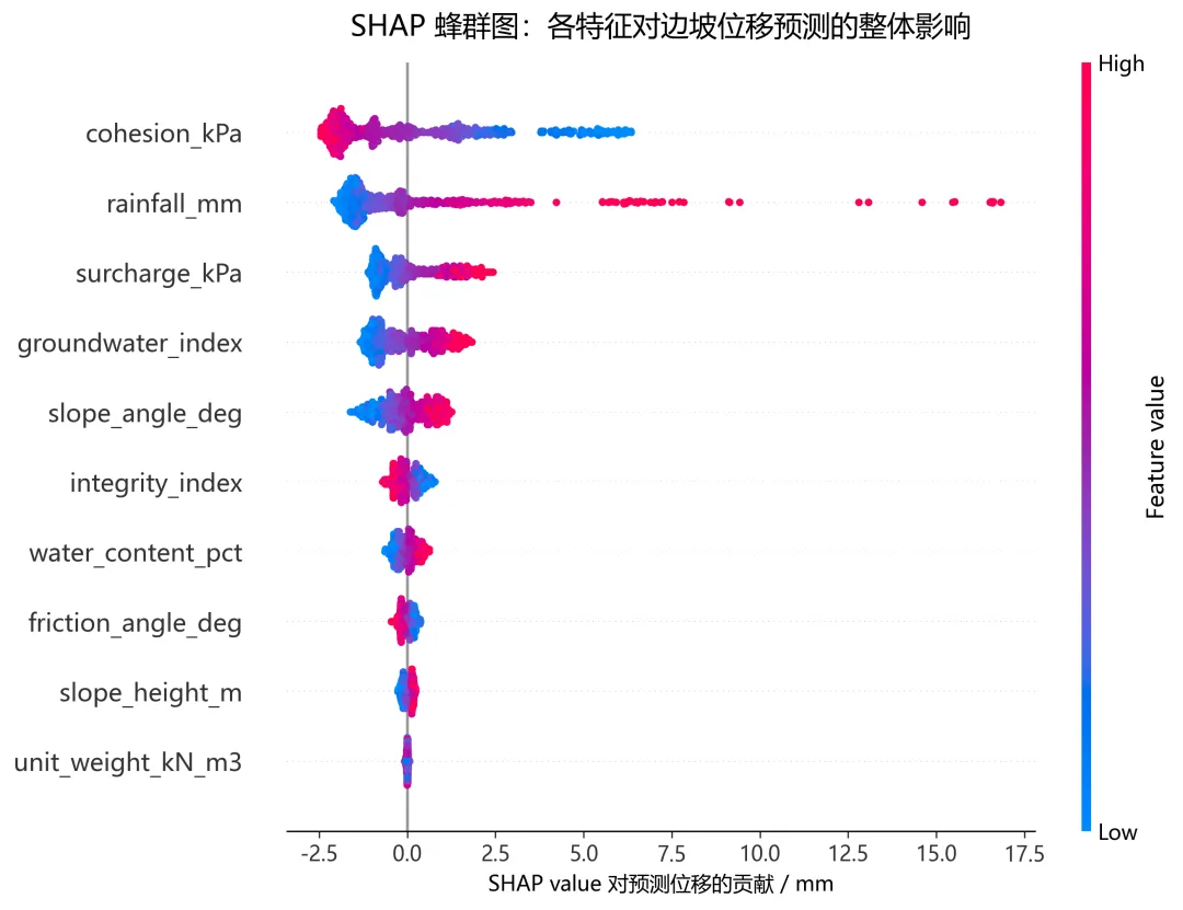
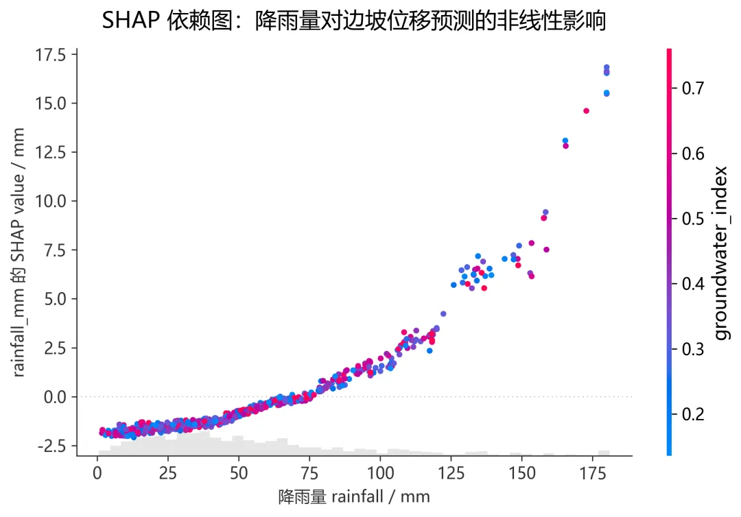
import osimport numpy as npimport pandas as pdimport matplotlib.pyplot as pltfrom sklearn.ensemble import RandomForestRegressorfrom sklearn.model_selection import train_test_splitfrom sklearn.metrics import r2_score, mean_squared_errorimport shapnp.random.seed(2026)plt.rcParams["font.sans-serif"] = ["Microsoft YaHei", "SimHei", "Arial Unicode MS", "DejaVu Sans"]plt.rcParams["axes.unicode_minus"] = Falseplt.rcParams["figure.dpi"] = 150plt.rcParams["savefig.dpi"] = 300out_dir = "SHAP_advanced_figures"os.makedirs(out_dir, exist_ok=True)N = 2500# 黏聚力 c，kPacohesion = np.random.normal(32, 7, N)cohesion = np.clip(cohesion, 10, 60)# 内摩擦角 phi，degreefriction_angle = np.random.normal(29, 4, N)friction_angle = np.clip(friction_angle, 16, 42)# 重度 gamma，kN/m3unit_weight = np.random.normal(19.2, 1.1, N)unit_weight = np.clip(unit_weight, 15.5, 23.0)# 含水率 water_content，%water_content = np.random.normal(18, 5, N)water_content = np.clip(water_content, 5, 38)# 坡角 slope_angle，degreeslope_angle = np.random.normal(36, 5, N)slope_angle = np.clip(slope_angle, 20, 55)# 降雨量 rainfall，mmrainfall = np.random.gamma(shape=2.0, scale=28.0, size=N)rainfall = np.clip(rainfall, 0, 180)# 坡高 slope_height，mslope_height = np.random.normal(28, 8, N)slope_height = np.clip(slope_height, 8, 60)# 外荷载 surcharge，kPasurcharge = np.random.gamma(shape=2.0, scale=10.0, size=N)surcharge = np.clip(surcharge, 0, 80)# 地下水位系数 groundwater，0~1groundwater = np.random.beta(2.5, 3.5, N)# 岩土体完整性指数 integrity，0~1integrity = np.random.beta(4.0, 2.0, N)# 构造一个带非线性和交互项的“真实位移”# 位移增大因素：降雨、坡角、坡高、含水率、地下水、外荷载# 位移减小因素：黏聚力、内摩擦角、完整性deformation = (    3.5    + 0.035 * rainfall    + 0.060 * slope_height    + 0.090 * surcharge    + 0.120 * water_content    + 0.180 * slope_angle    + 5.5 * groundwater    - 0.070 * cohesion    - 0.130 * friction_angle    - 3.8 * integrity)deformation += 0.0009 * np.maximum(rainfall - 70, 0) ** 2deformation += 0.018 * water_content * groundwater * rainfall / 20deformation += 0.010 * slope_angle * np.maximum(35 - cohesion, 0)deformation += np.random.normal(0, 1.4, N)deformation = np.clip(deformation, 0, None)df = pd.DataFrame({    "cohesion_kPa": cohesion,    "friction_angle_deg": friction_angle,    "unit_weight_kN_m3": unit_weight,    "water_content_pct": water_content,    "slope_angle_deg": slope_angle,    "rainfall_mm": rainfall,    "slope_height_m": slope_height,    "surcharge_kPa": surcharge,    "groundwater_index": groundwater,    "integrity_index": integrity,    "deformation_mm": deformation})# 3. 训练机器学习模型feature_cols = [    "cohesion_kPa",    "friction_angle_deg",    "unit_weight_kN_m3",    "water_content_pct",    "slope_angle_deg",    "rainfall_mm",    "slope_height_m",    "surcharge_kPa",    "groundwater_index",    "integrity_index"]X = df[feature_cols]y = df["deformation_mm"]X_train, X_test, y_train, y_test = train_test_split(    X, y,    test_size=0.25,    random_state=2026)model = RandomForestRegressor(    n_estimators=350,    max_depth=9,    min_samples_leaf=4,    random_state=2026,    n_jobs=-1)model.fit(X_train, y_train)y_pred = model.predict(X_test)r2 = r2_score(y_test, y_pred)rmse = np.sqrt(mean_squared_error(y_test, y_pred))print(f"R2 = {r2:.3f}")print(f"RMSE = {rmse:.3f} mm")# 4. 计算 SHAP 值sample_size = min(800, len(X_test))X_shap = X_test.sample(sample_size, random_state=2026)explainer = shap.TreeExplainer(model)shap_values = explainer(X_shap)# 5. 图1：SHAP 蜂群图plt.figure(figsize=(9.2, 6.8))shap.plots.beeswarm(    shap_values,    max_display=10,    show=False,    color_bar=True,    plot_size=None)plt.title(    "SHAP 蜂群图：各特征对边坡位移预测的整体影响",    fontsize=15,    pad=14)plt.xlabel("SHAP value 对预测位移的贡献 / mm", fontsize=11)plt.tight_layout()plt.savefig(    os.path.join(out_dir, "01_SHAP_beeswarm_slope_deformation.png"),    bbox_inches="tight")# 6. 图2：SHAP 依赖图#    这里选择 rainfall_mm 作为主变量#    用 groundwater_index 着色，展示交互效应plt.figure(figsize=(8.5, 6.3))shap.plots.scatter(    shap_values[:, "rainfall_mm"],    color=shap_values[:, "groundwater_index"],    show=False)plt.title(    "SHAP 依赖图：降雨量对边坡位移预测的非线性影响",    fontsize=15,    pad=14)plt.xlabel("降雨量 rainfall / mm", fontsize=11)plt.ylabel("rainfall_mm 的 SHAP value / mm", fontsize=11)plt.tight_layout()plt.savefig(    os.path.join(out_dir, "02_SHAP_dependence_rainfall_groundwater.png"),    bbox_inches="tight")# 7. 保存模拟数据和预测结果df.to_csv(    os.path.join(out_dir, "synthetic_geotechnical_monitoring_dataset.csv"),    index=False,    encoding="utf-8-sig")pred_df = X_test.copy()pred_df["y_true_deformation_mm"] = y_test.valuespred_df["y_pred_deformation_mm"] = y_predpred_df.to_csv(    os.path.join(out_dir, "prediction_results.csv"),    index=False,    encoding="utf-8-sig")

特别声明：

以上代码与文案均为网上资料整合而成，仅供广大同行们参考学习，如有侵权请联系删除。