机器学习--基础入门--07Python入门机器学习
- 2026-07-02 02:53:02
Python入门机器学习:从零到实战
欢迎来到机器学习的世界!在这个数据驱动的时代,Python已成为机器学习领域当之无愧的王者——简洁的语法、强大的生态、活跃的社区,让无数开发者爱不释手。但你是否曾困惑:环境怎么配置?库怎么安装?代码怎么写?
别担心,这一切我们都会解决。本章将带你完成从环境搭建到模型训练的完整旅程:安装Python与Anaconda、配置虚拟环境、掌握Jupyter Notebook、安装机器学习核心库,最后亲手实现一个鸢尾花分类项目。不只是"看懂",更要"动手做"。准备好了吗?让我们开始你的机器学习实战之旅!
第一章:Python环境安装
1.1 为什么选择Python?
Python之所以成为机器学习的首选语言,有三个核心优势:
| 优势 | 说明 | 举例 |
|---|---|---|
| 语法简洁 | 接近自然语言,易于学习 | <font style="color:rgb(0, 0, 0);">print("Hello ML!")</font> |
| 生态丰富 | 拥有大量成熟的机器学习库 | NumPy、Pandas、Scikit-learn、PyTorch |
| 社区活跃 | 遇到问题容易找到解决方案 | Stack Overflow上有海量Python问答 |
1.2 安装方法选择
Python主要有两种安装方式
方法一:官方安装器
适用场景:只需要Python运行环境,硬盘空间有限
Windows系统:
1 2 3 4 5 6 # 步骤1:访问 https://www.python.org/downloads/# 步骤2:下载最新稳定版(推荐3.10以上的版本)# 步骤3:运行安装程序,务必勾选以下选项# ⚠️ 重要:安装时必须勾选 "Add Python to PATH"# 这会将Python添加到系统环境变量,让你可以在任何位置运行Python
macOS系统:
1 2 3 4 5 6 7 8 9 10 11 # 方法1:官网下载 .pkg 文件双击安装# 方法2:使用Homebrew(推荐mac用户)# 首先安装Homebrew(如果还没有)/bin/bash -c "$(curl -fsSL https://raw.githubusercontent.com/Homebrew/install/HEAD/install.sh)"# 然后安装Pythonbrew install python3# 验证安装python3 --version
Linux系统:
1 2 3 4 5 6 7 8 9 10 # Ubuntu/Debiansudo apt updatesudo apt install python3 python3-pip python3-venv# CentOS/RHELsudo yum install python3 python3-pip# 验证安装python3 --versionpip3 --version
方法二:Anaconda发行版(强烈推荐初学者)
Anaconda是一个专为数据科学设计的Python发行版,预装了超过150个科学计算包。
Anaconda的核心优势:
安装步骤:
1 2 3 4 5 6 7 8 9 10 11 12 13 14 15 # 步骤1:访问官网# https://www.anaconda.com/products/distribution# 步骤2:下载对应操作系统的安装包# Windows: .exe 文件# macOS: .pkg 文件# Linux: .sh 文件# 步骤3:运行安装程序# Linux用户使用命令行安装:bash Anaconda3-2023.03-Linux-x86_64.sh# 步骤4:验证安装conda --version # 应显示 conda 版本号python --version # 应显示 Python 版本号
⚠️ 注意事项:
• 安装过程中会询问是否初始化conda,建议选择"yes" • Windows用户可能需要重启终端/命令提示符才能使用conda命令
第二章:虚拟环境管理
2.1 为什么需要虚拟环境?
🤔 问题场景:你正在开发两个项目:
• 项目A需要 NumPy 1.19 版本 • 项目B需要 NumPy 1.24 版本 如果只有一个Python环境,你该怎么办?
这就是虚拟环境要解决的核心问题:依赖隔离。
什么是依赖隔离?
想象一下,你在厨房做饭:
• 🍳 中式厨房:有特定的调料(豆瓣酱、生抽...) • 🍝 西式厨房:有另一套调料(橄榄油、罗勒叶...)
虚拟环境就像为每个项目准备的独立厨房,每个厨房可以有自己的"调料"(库版本),互不干扰。
虚拟环境的好处详解
| 依赖隔离 | ||
| 环境复现 | ||
| 权限管理 | ||
| 项目清理 | conda env remove -n project_name 彻底清理 | |
| 错误隔离 |
2.2 使用conda管理环境
conda是Anaconda自带的包和环境管理工具,功能强大且易用。
1 2 3 4 5 6 7 8 9 10 11 12 13 14 15 16 17 18 19 20 21 22 23 24 25 26 27 28 29 30 31 32 33 34 35 36 37 38 39 40 41 42 43 44 45 46 47 48 49 50 51 52 53 # 1️⃣ 创建虚拟环境# 语法:conda create -n 环境名 python=版本号conda create -n ml_env python=3.9# 执行后会询问是否继续,输入 y 确认# 2️⃣ 激活环境# Windows:conda activate ml_env# macOS/Linux:conda activate ml_env# 或 source activate ml_env# 激活后,终端提示符前会出现环境名# 3️⃣ 安装包# 在激活的环境中安装conda install numpy pandas matplotlib scikit-learn# 指定版本安装conda install numpy=1.21.0# 4️⃣ 查看已安装的包conda list# 5️⃣ 查看所有环境conda env list# 或conda info --envs# 6️⃣ 退出当前环境conda deactivate# 7️⃣ 删除环境conda env remove -n ml_env# 或conda remove -n ml_env --all# 🔹 导出环境配置(方便分享和复现)# 激活环境后执行:conda env export > environment.yml# 🔹 从配置文件创建环境conda env create -f environment.yml# 🔹 克隆现有环境conda create -n ml_env_copy --clone ml_env# 🔹 重命名环境(通过克隆+删除实现)conda create -n new_name --clone old_nameconda env remove -n old_name
2.3 conda vs pip 详细对比--conda和pip有什么区别?
| 来源 | ||
| 包来源 | ||
| 语言支持 | ||
| 依赖管理 | ||
| 环境管理 | ||
| 安装位置 | ||
| 二进制包 | ||
| 适用场景 |
最佳实践建议:
1 2 3 4 5 6 7 8 # 在conda环境中,优先使用conda安装conda install numpy pandas matplotlib# 如果conda仓库中没有某个包,再用pip安装pip install some-special-package# ⚠️ 注意:在conda环境中使用pip后,尽量避免再用conda更新包# 可能导致依赖关系混乱
2.4 创建机器学习专用环境
让我们创建一个适合本教程的完整环境:
1 2 3 4 5 6 7 8 9 10 11 12 # 创建名为ml_course的环境,使用Python 3.9conda create -n ml_course python=3.9 -y# 激活环境conda activate ml_course# 安装机器学习核心库conda install numpy pandas matplotlib seaborn scikit-learn jupyter -y# 验证安装python -c "import sklearn; print(f'scikit-learn版本: {sklearn.__version__}')"# 应输出版本号,如:scikit-learn版本: 1.2.2
第三章:开发工具配置
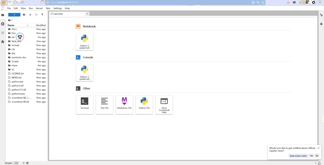
3.1 Jupyter Notebook
📓 Jupyter Notebook就像一本"活"的笔记本,你可以:
• 写文字记录想法 • 写代码并立即看到结果 • 插入图表和数据可视化
它是数据科学家最喜爱的开发工具之一,特别适合:
• 数据探索和分析 • 机器学习原型开发 • 教学和文档分享
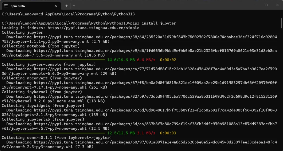
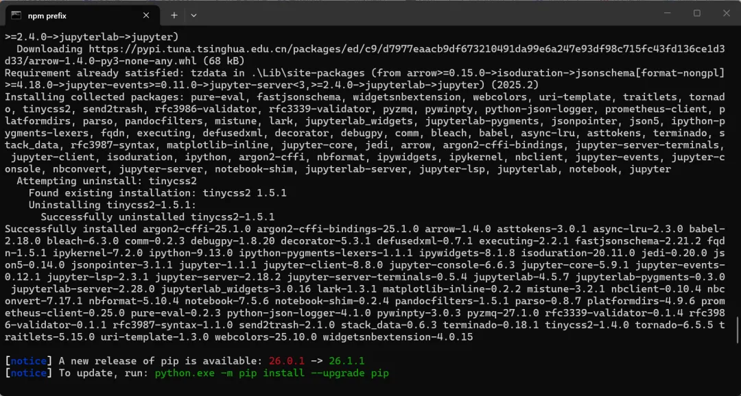
安装和启动 Jupyter
1 2 # 安装 Jupyterpip install jupyter
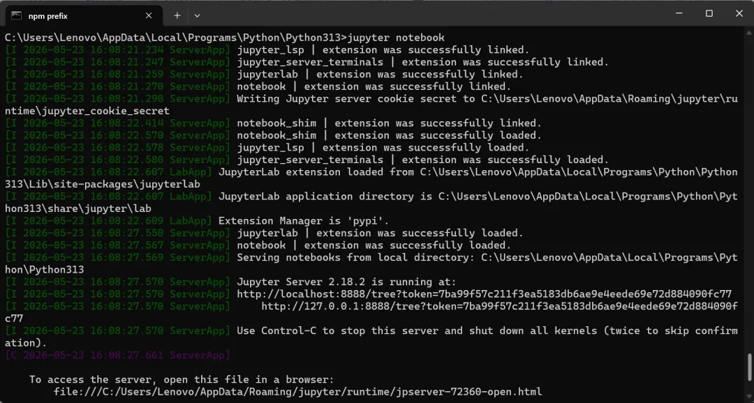
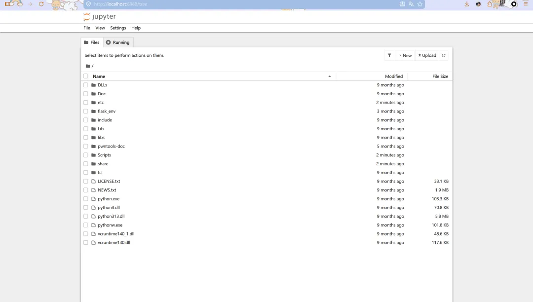
启动 Jupyter Notebook
1 jupyter notebook # 启动 Jupyter Notebook
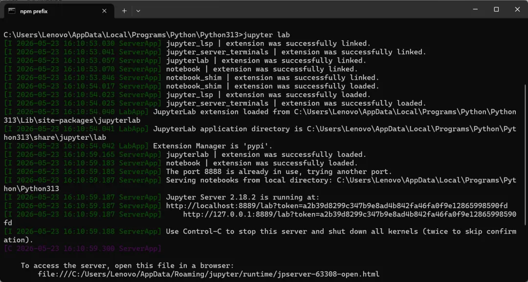
启动 Jupyter Lab(更现代的界面)
1 jupyter lab # 启动 Jupyter Lab(更现代的界面)
Jupyter基本使用
核心快捷键(务必记住!):
Shift + Enter | ||
Ctrl + Enter | ||
A | ||
B | ||
DD | ||
M | ||
Y | ||
Tab | ||
Shift + Tab |
单元格类型:
• Code单元格:写代码,运行后显示结果 • Markdown单元格:写文字、标题、列表等
实例1:学生成绩分析
让我们通过一个完整案例学习Jupyter的使用:
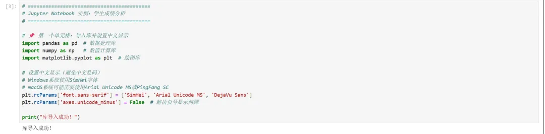
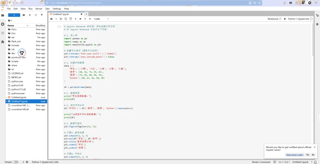
1 2 3 4 5 6 7 8 9 10 11 12 13 14 15 16 # ==========================================# Jupyter Notebook 实例:学生成绩分析# ==========================================# 📌 第一个单元格:导入库并设置中文显示import pandas as pd # 数据处理库import numpy as np # 数值计算库import matplotlib.pyplot as plt # 绘图库# 设置中文显示(避免中文乱码)# Windows系统使用SimHei字体# macOS系统可能需要使用Arial Unicode MS或PingFang SCplt.rcParams['font.sans-serif'] = ['SimHei', 'Arial Unicode MS', 'DejaVu Sans']plt.rcParams['axes.unicode_minus'] = False # 解决负号显示问题print("库导入成功!")
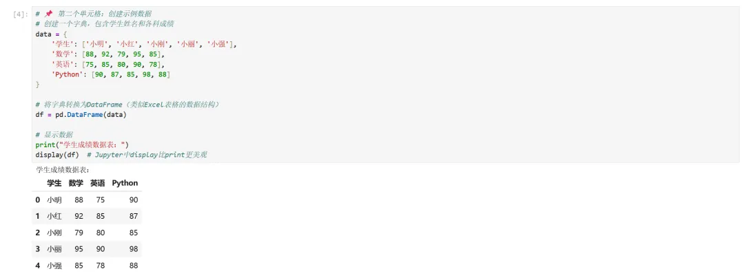
1 2 3 4 5 6 7 8 9 10 11 12 13 14 15 # 📌 第二个单元格:创建示例数据# 创建一个字典,包含学生姓名和各科成绩data = { '学生': ['小明', '小红', '小刚', '小丽', '小强'], '数学': [88, 92, 79, 95, 85], '英语': [75, 85, 80, 90, 78], 'Python': [90, 87, 85, 98, 88]}# 将字典转换为DataFrame(类似Excel表格的数据结构)df = pd.DataFrame(data)# 显示数据print("学生成绩数据表:")display(df) # Jupyter中display比print更美观
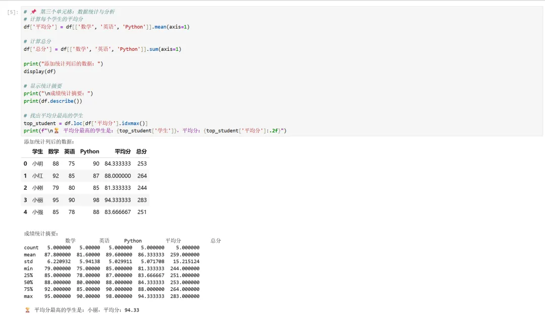
1 2 3 4 5 6 7 8 9 10 11 12 13 14 15 16 17 # 📌 第三个单元格:数据统计与分析# 计算每个学生的平均分df['平均分'] = df[['数学', '英语', 'Python']].mean(axis=1)# 计算总分df['总分'] = df[['数学', '英语', 'Python']].sum(axis=1)print("添加统计列后的数据:")display(df)# 显示统计摘要print("\n成绩统计摘要:")print(df.describe())# 找出平均分最高的学生top_student = df.loc[df['平均分'].idxmax()]print(f"\n🏆 平均分最高的学生是:{top_student['学生']},平均分:{top_student['平均分']:.2f}")
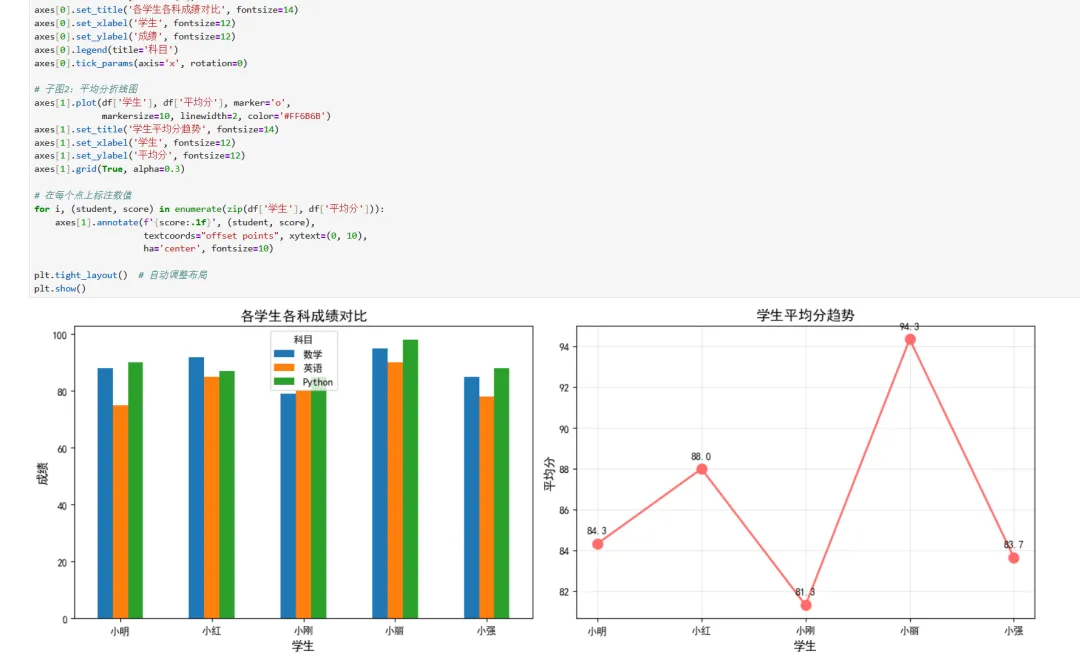
1 2 3 4 5 6 7 8 9 10 11 12 13 14 15 16 17 18 19 20 21 22 23 24 25 26 27 28 29 # 📌 第四个单元格:数据可视化# 创建一个画布,包含2个子图fig, axes = plt.subplots(1, 2, figsize=(14, 5))# 子图1:各科成绩柱状图df.plot(x='学生', y=['数学', '英语', 'Python'], kind='bar', ax=axes[0])axes[0].set_title('各学生各科成绩对比', fontsize=14)axes[0].set_xlabel('学生', fontsize=12)axes[0].set_ylabel('成绩', fontsize=12)axes[0].legend(title='科目')axes[0].tick_params(axis='x', rotation=0)# 子图2:平均分折线图axes[1].plot(df['学生'], df['平均分'], marker='o', markersize=10, linewidth=2, color='#FF6B6B')axes[1].set_title('学生平均分趋势', fontsize=14)axes[1].set_xlabel('学生', fontsize=12)axes[1].set_ylabel('平均分', fontsize=12)axes[1].grid(True, alpha=0.3)# 在每个点上标注数值for i, (student, score) in enumerate(zip(df['学生'], df['平均分'])): axes[1].annotate(f'{score:.1f}', (student, score), textcoords="offset points", xytext=(0, 10), ha='center', fontsize=10)plt.tight_layout() # 自动调整布局plt.show()
实例2:数据加载与简单清洗
在实际项目中,数据通常来自外部文件(CSV、Excel等),且往往需要清洗。让我们看一个更实际的例子:
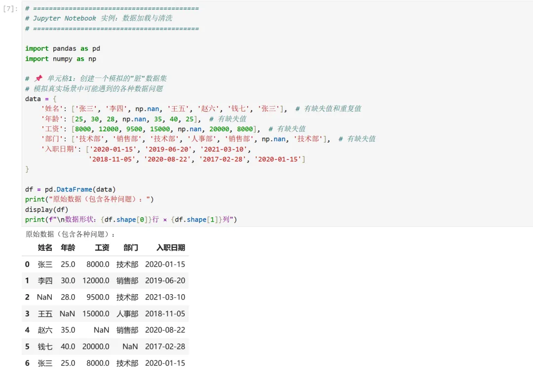
1 2 3 4 5 6 7 8 9 10 11 12 13 14 15 16 17 18 19 20 21 22 # ==========================================# Jupyter Notebook 实例:数据加载与清洗# ==========================================import pandas as pdimport numpy as np# 📌 单元格1:创建一个模拟的"脏"数据集# 模拟真实场景中可能遇到的各种数据问题data = { '姓名': ['张三', '李四', np.nan, '王五', '赵六', '钱七', '张三'], # 有缺失值和重复值 '年龄': [25, 30, 28, np.nan, 35, 40, 25], # 有缺失值 '工资': [8000, 12000, 9500, 15000, np.nan, 20000, 8000], # 有缺失值 '部门': ['技术部', '销售部', '技术部', '人事部', '销售部', np.nan, '技术部'], # 有缺失值 '入职日期': ['2020-01-15', '2019-06-20', '2021-03-10', '2018-11-05', '2020-08-22', '2017-02-28', '2020-01-15']}df = pd.DataFrame(data)print("原始数据(包含各种问题):")display(df)print(f"\n数据形状:{df.shape[0]}行 × {df.shape[1]}列")
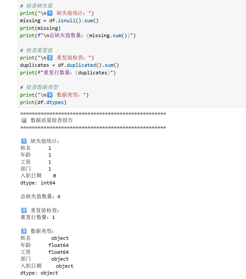
1 2 3 4 5 6 7 8 9 10 11 12 13 14 15 16 17 18 19 # 📌 单元格2:数据质量检查print("=" * 50)print("📊 数据质量检查报告")print("=" * 50)# 检查缺失值print("\n1️⃣ 缺失值统计:")missing = df.isnull().sum()print(missing)print(f"\n总缺失值数量:{missing.sum()}")# 检查重复值print("\n2️⃣ 重复值检查:")duplicates = df.duplicated().sum()print(f"重复行数量:{duplicates}")# 检查数据类型print("\n3️⃣ 数据类型:")print(df.dtypes)
1 2 3 4 5 6 7 8 9 10 11 12 13 14 15 16 17 18 19 20 21 22 23 24 25 26 27 # 📌 单元格3:数据清洗print("🧹 开始数据清洗...\n")# 步骤1:删除完全重复的行df_cleaned = df.drop_duplicates()print(f"删除重复行后:{df_cleaned.shape[0]}行")# 步骤2:处理缺失值# 对于数值列(年龄、工资),用中位数填充df_cleaned['年龄'].fillna(df_cleaned['年龄'].median(), inplace=True)df_cleaned['工资'].fillna(df_cleaned['工资'].median(), inplace=True)# 对于分类列(部门),用众数填充df_cleaned['部门'].fillna(df_cleaned['部门'].mode()[0], inplace=True)# 对于姓名缺失的行,直接删除(关键信息不能补)df_cleaned = df_cleaned.dropna(subset=['姓名'])print(f"处理缺失值后:{df_cleaned.shape[0]}行")# 步骤3:转换数据类型df_cleaned['入职日期'] = pd.to_datetime(df_cleaned['入职日期'])print("\n✅ 清洗后的数据:")display(df_cleaned)print(f"\n数据类型:")print(df_cleaned.dtypes)
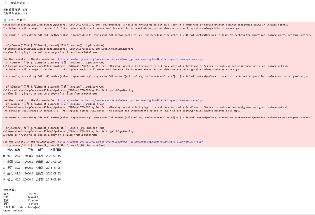
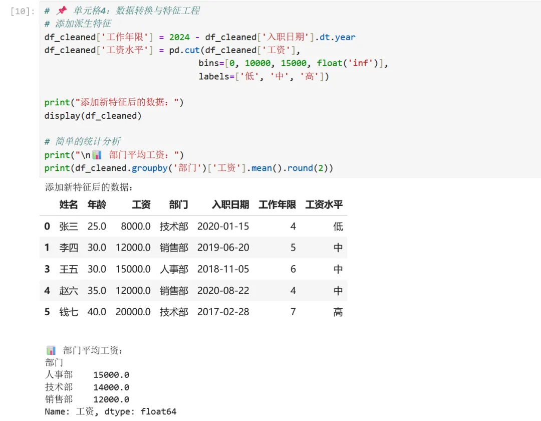
1 2 3 4 5 6 7 8 9 10 11 12 13 # 📌 单元格4:数据转换与特征工程# 添加派生特征df_cleaned['工作年限'] = 2024 - df_cleaned['入职日期'].dt.yeardf_cleaned['工资水平'] = pd.cut(df_cleaned['工资'], bins=[0, 10000, 15000, float('inf')], labels=['低', '中', '高'])print("添加新特征后的数据:")display(df_cleaned)# 简单的统计分析print("\n📊 部门平均工资:")print(df_cleaned.groupby('部门')['工资'].mean().round(2))
实例3学生成绩分析示例
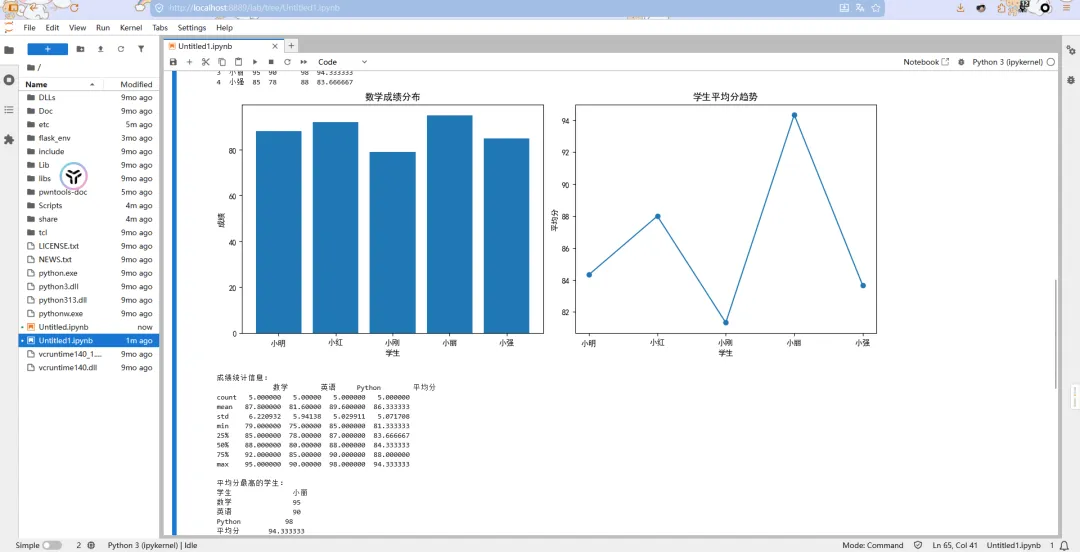
1 2 3 4 5 6 7 8 9 10 11 12 13 14 15 16 17 18 19 20 21 22 23 24 25 26 27 28 29 30 31 32 33 34 35 36 37 38 39 40 41 42 43 44 45 46 47 48 49 50 51 52 53 54 55 56 57 58 59 60 61 62 63 64 # 在 Jupyter Notebook 中运行以下代码# 1. 导入库import pandas as pdimport numpy as npimport matplotlib.pyplot as plt# 设置中文显示(避免中文乱码)plt.rcParams['font.sans-serif'] = ['SimHei']plt.rcParams['axes.unicode_minus'] = False# 2. 创建示例数据data = { '学生': ['小明', '小红', '小刚', '小丽', '小强'], '数学': [88, 92, 79, 95, 85], '英语': [75, 85, 80, 90, 78], 'Python': [90, 87, 85, 98, 88]}df = pd.DataFrame(data)# 3. 数据预览print("学生成绩数据:")print(df)# 4. 添加平均分列df['平均分'] = df[['数学', '英语', 'Python']].mean(axis=1)print("\n添加平均分后的数据:")print(df)# 5. 数据可视化plt.figure(figsize=(12, 5))# 子图1:数学成绩plt.subplot(1, 2, 1)plt.bar(df['学生'], df['数学'])plt.title('数学成绩分布')plt.xlabel('学生')plt.ylabel('成绩')# 子图2:平均分plt.subplot(1, 2, 2)plt.plot(df['学生'], df['平均分'], marker='o')plt.title('学生平均分趋势')plt.xlabel('学生')plt.ylabel('平均分')plt.tight_layout()plt.show()# 6. 统计分析print("\n成绩统计信息:")print(df.describe())# 7. 找出平均分最高的学生top_student = df.loc[df['平均分'].idxmax()]print("\n平均分最高的学生:")print(top_student)# 8. 各科平均成绩print("\n各科平均成绩:")print(df[['数学', '英语', 'Python']].mean())
3.2 VS Code配置
Visual Studio Code是一个轻量级但功能强大的代码编辑器,通过安装插件可以成为专业的机器学习开发环境。
安装VS Code
1. 访问官网:https://code.visualstudio.com/ 2. 下载对应操作系统的版本 3. 安装时建议勾选"添加到右键菜单"等选项
插件清单
| Python | |
| Jupyter | |
| Pylance | |
| Python Indent | |
| autoDocstring | |
| GitLens | |
| Rainbow Brackets | |
| Code Runner |
代码质量工具配置
除了编辑器插件,还需要安装代码检查和格式化工具:
1 2 3 4 5 6 7 8 # 安装代码检查工具pip install flake8 pylint# 安装代码格式化工具pip install black autopep8# 安装类型检查工具(可选)pip install mypy
VS Code配置详解
在项目根目录创建 .vscode/settings.json 文件:
1 2 3 4 5 6 7 8 9 10 11 12 13 14 15 16 17 18 19 20 21 22 23 24 25 26 27 28 29 30 31 32 33 34 35 36 37 38 39 40 41 42 43 44 45 46 47 48 49 50 51 52 { // ==================== Python配置 ==================== // Python解释器路径(使用conda环境) "python.defaultInterpreterPath": "${workspaceFolder}/envs/ml_course/bin/python", // 代码检查配置 "python.linting.enabled":true, "python.linting.pylintEnabled":true, "python.linting.flake8Enabled":true, "python.linting.flake8Args": [ "--max-line-length=120", // 最大行长度 "--ignore=E501,W503" // 忽略的检查项 ], // 代码格式化配置 "python.formatting.provider": "black", "editor.formatOnSave":true, // 保存时自动格式化 "python.formatting.blackArgs": [ "--line-length=120" ], // 测试配置 "python.testing.pytestEnabled":true, "python.testing.unittestEnabled":false, // ==================== Jupyter配置 ==================== "jupyter.askForKernelRestart":false, // 重启内核不询问 "jupyter.runStartupCommands": [ "import pandas as pd\nimport numpy as np" ], // ==================== 编辑器配置 ==================== "editor.fontSize": 14, "editor.tabSize": 4, "editor.insertSpaces":true, "editor.wordWrap": "on", "editor.minimap.enabled":false, // 文件自动保存 "files.autoSave": "afterDelay", "files.autoSaveDelay": 1000, // 终端配置 "terminal.integrated.fontSize": 13, // 文件排除 "files.exclude": { "**/__pycache__":true, "**/*.pyc":true, "**/.ipynb_checkpoints":true }}
第四章:机器学习库安装
4.1 核心库介绍
| NumPy | ||
| Pandas | ||
| Matplotlib | ||
| Seaborn | ||
| Scikit-learn | ||
| Jupyter |
4.2 安装命令
1 2 3 4 5 6 7 8 9 10 11 12 13 # 激活虚拟环境conda activate ml_course# 安装核心机器学习库(推荐使用conda)conda install numpy pandas matplotlib seaborn scikit-learn jupyter -y# 或者使用pip安装pip install numpy pandas matplotlib seaborn scikit-learn jupyter# 验证安装python -c "import numpy; print(f'NumPy: {numpy.__version__}')"python -c "import pandas; print(f'Pandas: {pandas.__version__}')"python -c "import sklearn; print(f'Scikit-learn: {sklearn.__version__}')"
4.3 深度学习框架
如果你打算学习深度学习:
1 2 3 4 5 6 7 8 9 # PyTorch(推荐初学者)# 访问 https://pytorch.org/ 获取适合你系统的安装命令# CPU版本:pip install torch torchvision torchaudio# TensorFlowpip install tensorflow# 注意:深度学习框架较大,建议在有需要时再安装
4.4 查看已安装库及版本
1 2 3 4 5 6 7 8 9 10 11 12 13 14 15 # 在Python中运行import pkg_resources# 获取已安装的包列表installed_packages = pkg_resources.working_setinstalled_packages_list = sorted(["%s==%s" % (i.key, i.version) for i in installed_packages])# 打印常用的机器学习库版本packages_of_interest = ['numpy', 'pandas', 'matplotlib', 'seaborn', 'scikit-learn']print("已安装的核心库版本:")for pkg in installed_packages_list: name = pkg.split('==')[0] if name in packages_of_interest: print(f" {pkg}")
第五章:机器学习实战 - 鸢尾花分类
经典的鸢尾花分类问题,体验完整机器学习的端到端流程。
5.1 机器学习工作流程概览
在开始编码之前,让我们先理解机器学习的标准工作流程:
1 2 3 4 5 ┌─────────────┐ ┌─────────────┐ ┌─────────────┐ ┌─────────────┐│ 数据获取 │ -> │ 数据预处理 │ -> │ 模型训练 │ -> │ 模型评估 │└─────────────┘ └─────────────┘ └─────────────┘ └─────────────┘ ↑ │ └───────────────── 模型优化(迭代) ←────────────────────────┘
5.2 步骤1:导入库
1 2 3 4 5 6 7 8 9 import pandas as pdimport matplotlib.pyplot as pltimport seaborn as snsfrom sklearn.datasets import load_iris# 设置绘图样式sns.set_style("whitegrid")plt.rcParams['font.sans-serif'] = ['SimHei', 'Arial Unicode MS']plt.rcParams['axes.unicode_minus'] = False
5.3步骤2:加载数据
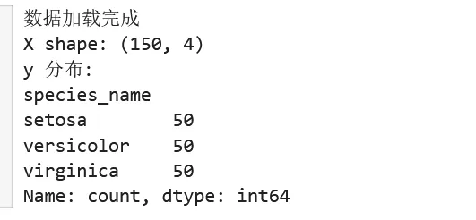
1 2 3 4 5 6 7 8 9 iris = load_iris()X = pd.DataFrame(iris.data, columns=iris.feature_names)y = pd.Series(iris.target, name='species')y_names = pd.Series([iris.target_names[i] for i in y], name='species_name')print("数据加载完成")print(f"X shape: {X.shape}")print(f"y 分布:\n{y_names.value_counts()}")
5.4 步骤3:
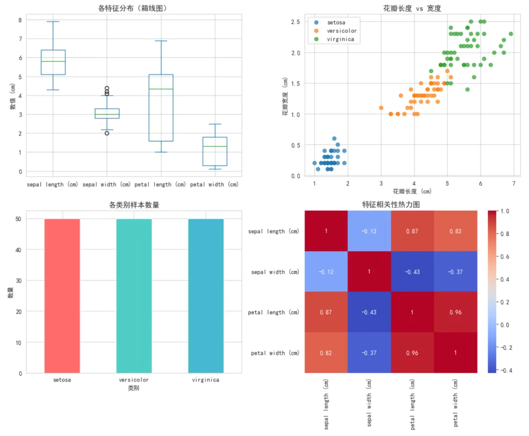
1 2 3 4 5 6 7 8 9 10 11 12 13 14 15 16 17 18 19 20 21 22 23 24 25 26 27 28 29 30 31 32 fig, axes = plt.subplots(2, 2, figsize=(12, 10))# 子图1:特征分布箱线图X.plot(kind='box', ax=axes[0, 0])axes[0, 0].set_title('各特征分布(箱线图)', fontsize=12)axes[0, 0].set_ylabel('数值 (cm)')# 子图2:散点图(花瓣长度 vs 宽度)for i, species in enumerate(iris.target_names): mask = y == i axes[0, 1].scatter(X.loc[mask, 'petal length (cm)'], X.loc[mask, 'petal width (cm)'], label=species, alpha=0.7)axes[0, 1].set_xlabel('花瓣长度 (cm)')axes[0, 1].set_ylabel('花瓣宽度 (cm)')axes[0, 1].set_title('花瓣长度 vs 宽度', fontsize=12)axes[0, 1].legend()# 子图3:类别分布柱状图y_names.value_counts().plot(kind='bar', ax=axes[1, 0], color=['#FF6B6B', '#4ECDC4', '#45B7D1'])axes[1, 0].set_title('各类别样本数量', fontsize=12)axes[1, 0].set_xlabel('类别')axes[1, 0].set_ylabel('数量')axes[1, 0].tick_params(axis='x', rotation=0)# 子图4:特征相关性热力图correlation = X.corr()sns.heatmap(correlation, annot=True, cmap='coolwarm', ax=axes[1, 1])axes[1, 1].set_title('特征相关性热力图', fontsize=12)plt.tight_layout()plt.show()
5.4 步骤3:数据集划分
为什么要划分训练集和测试集?
概念就是模型评估的"公平性"
例如你在备考:
• 📚 训练集:复习资料(用来学习) • 📝 测试集:考试题目(用来检验真实水平)
如果考试题目和复习资料一样,那考高分不能证明你真的学会了。同样,如果用训练数据来测试模型,模型可能只是"死记硬背"了答案,而不是真正学会了规律。
训练集/测试集划分的意义:
• 训练集:用于训练模型,让模型学习数据中的规律 • 测试集:用于评估模型,测试模型在未见数据上的表现 • 防止过拟合:如果模型在训练集上表现很好但测试集很差,说明模型"过拟合"了
随机种子(random_state)的作用
1 2 3 4 5 6 7 8 # 每次运行结果不同X_train, X_test, y_train, y_test = train_test_split(X, y, test_size=0.2)# 第一次运行可能得到:测试集样本 [12, 45, 78, ...]# 第二次运行可能得到:测试集样本 [23, 67, 89, ...]# 使用random_state保证结果可复现X_train, X_test, y_train, y_test = train_test_split(X, y, test_size=0.2, random_state=42)# 每次运行都得到相同的划分结果
为什么需要random_state?
1. 结果可复现:别人运行你的代码能得到相同结果 2. 调试方便:确保每次测试使用相同的数据 3. 公平比较:比较不同模型时使用相同的数据划分
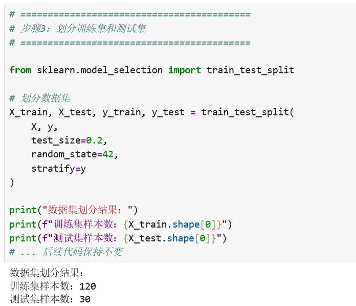
1 2 3 4 5 6 7 8 9 10 11 12 13 14 15 16 17 18 # ==========================================# 步骤3:划分训练集和测试集# ==========================================from sklearn.model_selection import train_test_split# 划分数据集X_train, X_test, y_train, y_test = train_test_split( X, y, test_size=0.2, random_state=42, stratify=y)print("数据集划分结果:")print(f"训练集样本数:{X_train.shape[0]}")print(f"测试集样本数:{X_test.shape[0]}")# ... 后续代码保持不变
5.5 步骤4:特征缩放(标准化)
什么是特征缩放?
📏 问题场景:假设有两个特征:
• 特征A:身高,范围150-200厘米 • 特征B:收入,范围5000-50000元 在计算距离时,收入的数值差异会主导距离计算,导致身高特征几乎被忽略。
标准化是将特征缩放到均值为0、标准差为1的分布。
数学公式:
其中:
• :原始值 • :特征的均值 • :特征的标准差 • :标准化后的值
为什么KNN特别需要标准化?
KNN算法基于距离:它通过计算样本之间的距离来判断相似性。
1 2 3 4 5 6 7 8 9 10 11 # 不标准化时的距离计算示例样本1: [身高=160cm, 收入=10000元]样本2: [身高=170cm, 收入=15000元]# 欧氏距离distance = sqrt((160-170)² + (10000-15000)²) = sqrt(100 + 25000000) = sqrt(25000100) ≈ 5000# 身高差异(10)在总距离中几乎可以忽略!
标准化后:
1 2 3 4 5 6 7 8 9 10 # 标准化后(均值=0,标准差=1)样本1: [身高=-1.2, 收入=-0.5]样本2: [身高=0.8, 收入=0.5]distance = sqrt((-1.2-0.8)² + (-0.5-0.5)²) = sqrt(4 + 1) = sqrt(5) ≈ 2.24# 两个特征对距离的贡献更均衡
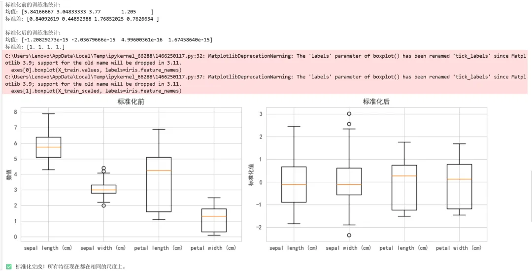
1 2 3 4 5 6 7 8 9 10 11 12 13 14 15 16 17 18 19 20 21 22 23 24 25 26 27 28 29 30 31 32 33 34 35 36 37 38 39 40 41 42 43 44 # ==========================================# 步骤4:特征标准化# ==========================================# 创建标准化器scaler = StandardScaler()# ⚠️ 重要:只在训练集上fit,然后用相同的参数转换训练集和测试集# fit:计算均值和标准差# transform:应用标准化# fit_transform:先计算再应用# 训练集:fit_transform(学习参数并转换)X_train_scaled = scaler.fit_transform(X_train)# 测试集:transform(使用训练集的参数转换)X_test_scaled = scaler.transform(X_test)# 查看标准化前后的对比print("标准化前的训练集统计:")print(f"均值:{X_train.mean().values}")print(f"标准差:{X_train.std().values}")print("\n标准化后的训练集统计:")print(f"均值:{X_train_scaled.mean(axis=0)}") # 应该接近0print(f"标准差:{X_train_scaled.std(axis=0)}") # 应该接近1# 可视化对比fig, axes = plt.subplots(1, 2, figsize=(12, 4))# 标准化前axes[0].boxplot(X_train.values, labels=iris.feature_names)axes[0].set_title('标准化前', fontsize=12)axes[0].set_ylabel('数值')# 标准化后axes[1].boxplot(X_train_scaled, labels=iris.feature_names)axes[1].set_title('标准化后', fontsize=12)axes[1].set_ylabel('标准化值')plt.tight_layout()plt.show()print("\n✅ 标准化完成!所有特征现在都在相同的尺度上。")
5.6 步骤5:KNN算法原理
在训练模型之前,让我们深入理解KNN算法。
KNN的核心思想
KNN(K-Nearest Neighbors,K近邻)是最简单直观的机器学习算法之一:
1. 训练阶段:只是"记住"所有训练数据(懒惰学习) 2. 预测阶段: • 计算新样本与所有训练样本的距离 • 找出距离最近的K个邻居 • 统计这K个邻居的类别 • 将新样本分类为出现次数最多的类别
工作流程图:
1 2 3 4 5 新样本 → 计算距离 → 找K个最近邻居 → 投票决定类别 ↓ [邻居1: 类别A] [邻居2: 类别A] [邻居3: 类别B] → K=3 → 类别A(2票)vs 类别B(1票)→ 预测:类别A
K值的选择
经验法则:K通常取奇数,避免平票;一般取 左右(n为样本数)
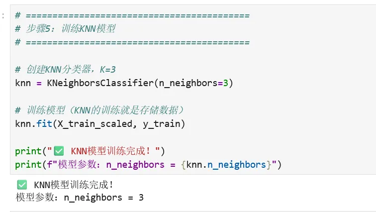
1 2 3 4 5 6 7 8 9 10 11 12 # ==========================================# 步骤5:训练KNN模型# ==========================================# 创建KNN分类器,K=3knn = KNeighborsClassifier(n_neighbors=3)# 训练模型(KNN的训练就是存储数据)knn.fit(X_train_scaled, y_train)print("✅ KNN模型训练完成!")print(f"模型参数:n_neighbors = {knn.n_neighbors}")
5.7 步骤6:模型评估
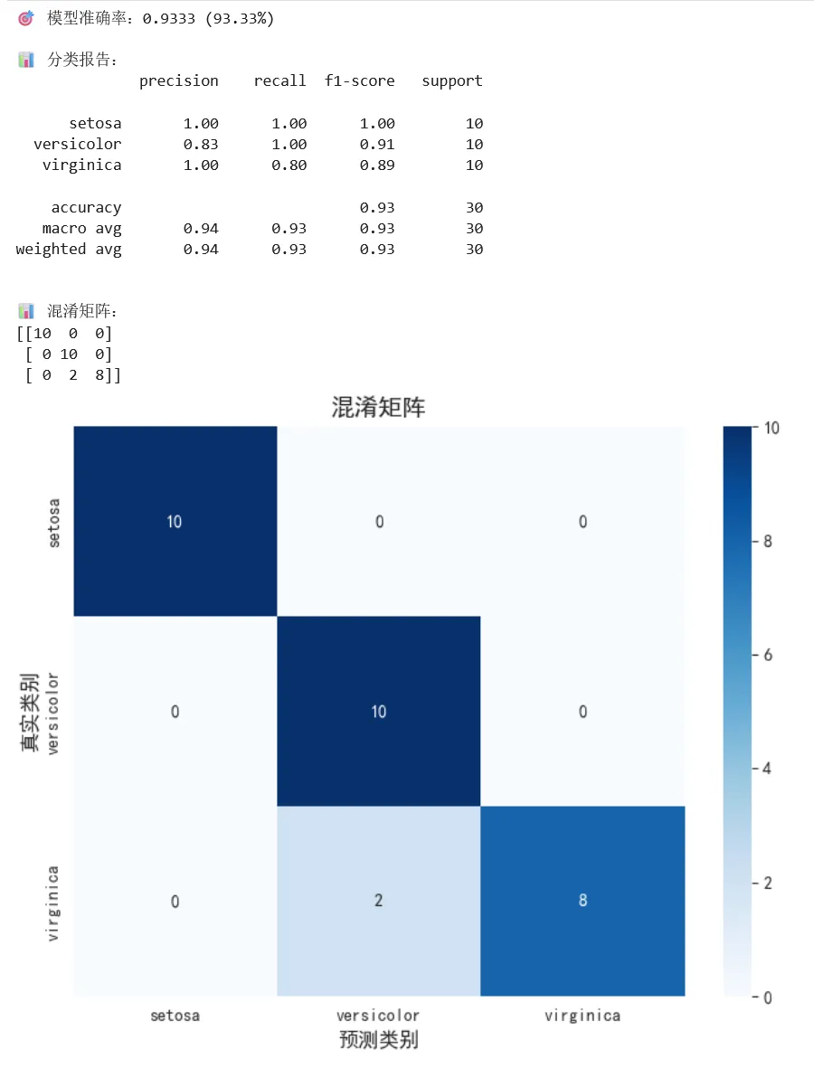
1 2 3 4 5 6 7 8 9 10 11 12 13 14 15 16 17 18 19 20 21 22 23 24 25 26 27 28 29 # ==========================================# 步骤6:评估模型# ==========================================# 在测试集上进行预测y_pred = knn.predict(X_test_scaled)# 计算准确率accuracy = accuracy_score(y_test, y_pred)print(f"🎯 模型准确率:{accuracy:.4f} ({accuracy*100:.2f}%)")# 详细的分类报告print("\n📊 分类报告:")print(classification_report(y_test, y_pred, target_names=iris.target_names))# 混淆矩阵print("\n📊 混淆矩阵:")cm = confusion_matrix(y_test, y_pred)print(cm)# 可视化混淆矩阵plt.figure(figsize=(8, 6))sns.heatmap(cm, annot=True, fmt='d', cmap='Blues', xticklabels=iris.target_names, yticklabels=iris.target_names)plt.title('混淆矩阵', fontsize=14)plt.xlabel('预测类别', fontsize=12)plt.ylabel('真实类别', fontsize=12)plt.show()
5.8 扩展:K值选择与准确率曲线
让我们通过实验找到最优的K值:
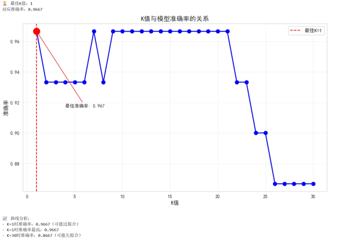
1 2 3 4 5 6 7 8 9 10 11 12 13 14 15 16 17 18 19 20 21 22 23 24 25 26 27 28 29 30 31 32 33 34 35 36 37 38 39 40 41 42 43 44 45 46 47 48 # ==========================================# 扩展:K值选择实验# ==========================================# 测试不同的K值k_range = range(1, 31) # 测试K从1到30k_scores = []for k in k_range: knn = KNeighborsClassifier(n_neighbors=k) knn.fit(X_train_scaled, y_train) y_pred = knn.predict(X_test_scaled) score = accuracy_score(y_test, y_pred) k_scores.append(score)# 找出最佳K值best_k = k_range[np.argmax(k_scores)]best_score = max(k_scores)print(f"🏆 最佳K值:{best_k}")print(f"对应准确率:{best_score:.4f}")# 绘制K值与准确率的关系曲线plt.figure(figsize=(10, 6))plt.plot(k_range, k_scores, 'bo-', linewidth=2, markersize=8)plt.axvline(x=best_k, color='r', linestyle='--', label=f'最佳K={best_k}')plt.scatter([best_k], [best_score], color='red', s=200, zorder=5)plt.xlabel('K值', fontsize=12)plt.ylabel('准确率', fontsize=12)plt.title('K值与模型准确率的关系', fontsize=14)plt.grid(True, alpha=0.3)plt.legend(fontsize=11)# 标注最佳点plt.annotate(f'最佳准确率: {best_score:.3f}', xy=(best_k, best_score), xytext=(best_k+3, best_score-0.05), fontsize=10, arrowprops=dict(arrowstyle='->', color='red'))plt.tight_layout()plt.show()# 分析曲线趋势print("\n📈 曲线分析:")print(f"- K=1时准确率:{k_scores[0]:.4f}(可能过拟合)")print(f"- K={best_k}时准确率最高:{best_score:.4f}")print(f"- K=30时准确率:{k_scores[-1]:.4f}(可能欠拟合)")
5.9 扩展:模型保存与加载
在实际项目中,我们需要保存训练好的模型,以便日后使用。
1 2 3 4 5 6 7 8 9 10 11 12 13 14 15 16 17 18 19 20 # ==========================================# 扩展:模型保存与加载# ==========================================import joblib # 或使用 pickleimport os# 创建模型保存目录model_dir = 'saved_models'os.makedirs(model_dir, exist_ok=True)# 保存模型和标准化器(⚠️ 重要:标准化器也要保存!)model_path = os.path.join(model_dir, 'knn_iris_model.pkl')scaler_path = os.path.join(model_dir, 'scaler.pkl')joblib.dump(knn, model_path)joblib.dump(scaler, scaler_path)print(f"✅ 模型已保存至:{model_path}")print(f"✅ 标准化器已保存至:{scaler_path}")

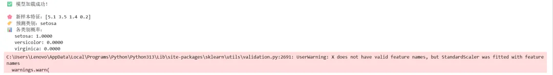
1 2 3 4 5 6 7 8 9 10 11 12 13 14 15 16 17 18 19 20 21 22 23 24 25 # 加载模型并预测新数据# 模拟真实应用场景# 加载保存的模型和标准化器loaded_knn = joblib.load(model_path)loaded_scaler = joblib.load(scaler_path)print("✅ 模型加载成功!")# 预测新样本# 假设我们在野外采集了一朵鸢尾花,测量结果如下:new_flower = np.array([[5.1, 3.5, 1.4, 0.2]]) # [花萼长, 花萼宽, 花瓣长, 花瓣宽]# ⚠️ 重要:必须使用训练时的标准化器进行相同的变换new_flower_scaled = loaded_scaler.transform(new_flower)# 预测prediction = loaded_knn.predict(new_flower_scaled)prediction_proba = loaded_knn.predict_proba(new_flower_scaled)print(f"\n🌸 新样本特征:{new_flower[0]}")print(f"🏷️ 预测类别:{iris.target_names[prediction[0]]}")print(f"📊 各类别概率:")for i, name in enumerate(iris.target_names): print(f" {name}: {prediction_proba[0][i]:.4f}")
5.10 完整代码汇总
1 2 3 4 5 6 7 8 9 10 11 12 13 14 15 16 17 18 19 20 21 22 23 24 25 26 27 28 29 30 31 32 33 34 35 36 37 38 39 40 41 42 43 44 45 46 47 48 49 50 51 52 53 54 55 56 57 58 59 60 61 62 63 64 65 66 67 68 # ==========================================# 完整代码:鸢尾花分类项目# ==========================================# ===== 1. 导入库 =====import numpy as npimport pandas as pdimport matplotlib.pyplot as pltimport seaborn as snsfrom sklearn.datasets import load_irisfrom sklearn.model_selection import train_test_splitfrom sklearn.preprocessing import StandardScalerfrom sklearn.neighbors import KNeighborsClassifierfrom sklearn.metrics import accuracy_score, classification_report, confusion_matriximport joblibimport warningswarnings.filterwarnings('ignore')# 中文显示设置plt.rcParams['font.sans-serif'] = ['SimHei', 'Arial Unicode MS']plt.rcParams['axes.unicode_minus'] = False# ===== 2. 加载数据 =====iris = load_iris()X = pd.DataFrame(iris.data, columns=iris.feature_names)y = pd.Series(iris.target, name='species')# ===== 3. 划分数据集 =====X_train, X_test, y_train, y_test = train_test_split( X, y, test_size=0.2, random_state=42, stratify=y)# ===== 4. 特征标准化 =====scaler = StandardScaler()X_train_scaled = scaler.fit_transform(X_train)X_test_scaled = scaler.transform(X_test)# ===== 5. 寻找最佳K值 =====k_range = range(1, 31)k_scores = []for k in k_range: knn = KNeighborsClassifier(n_neighbors=k) knn.fit(X_train_scaled, y_train) k_scores.append(accuracy_score(y_test, knn.predict(X_test_scaled)))best_k = k_range[np.argmax(k_scores)]print(f"最佳K值:{best_k}")# ===== 6. 训练最终模型 =====final_knn = KNeighborsClassifier(n_neighbors=best_k)final_knn.fit(X_train_scaled, y_train)# ===== 7. 评估模型 =====y_pred = final_knn.predict(X_test_scaled)print(f"\n模型准确率:{accuracy_score(y_test, y_pred):.4f}")print("\n分类报告:")print(classification_report(y_test, y_pred, target_names=iris.target_names))# ===== 8. 保存模型 =====joblib.dump(final_knn, 'saved_models/knn_iris_model.pkl')joblib.dump(scaler, 'saved_models/scaler.pkl')print("\n✅ 模型保存完成!")# ===== 9. 预测新样本 =====new_sample = np.array([[5.9, 3.0, 5.1, 1.8]])new_sample_scaled = scaler.transform(new_sample)prediction = final_knn.predict(new_sample_scaled)print(f"\n新样本预测结果:{iris.target_names[prediction[0]]}")
第六章:常见问题与解决方案(FAQ)
Q1:安装库时网络慢/失败怎么办?
问题描述:使用pip或conda安装库时速度很慢,甚至超时失败。
解决方案:
方法1:使用国内镜像源
1 2 3 4 5 6 7 8 9 10 # pip使用清华镜像pip install numpy -i https://pypi.tuna.tsinghua.edu.cn/simple# 永久配置pip镜像pip config set global.index-url https://pypi.tuna.tsinghua.edu.cn/simple# conda使用清华镜像conda config --add channels https://mirrors.tuna.tsinghua.edu.cn/anaconda/pkgs/mainconda config --add channels https://mirrors.tuna.tsinghua.edu.cn/anaconda/pkgs/freeconda config --set show_channel_urls yes
常用镜像源:
方法2:离线安装
1 2 3 4 5 6 7 # 1. 在有网络的电脑上下载whl文件# 访问 https://pypi.org/ 或 https://www.lfd.uci.edu/~gohlke/pythonlibs/# 2. 将whl文件复制到目标电脑# 3. 离线安装pip install /path/to/package.whl
Q2:启动Jupyter时端口被占用怎么办?
问题描述:运行 jupyter notebook 时提示端口8888已被占用。
解决方案:
方法1:指定其他端口
1 2 # 使用其他端口启动jupyter notebook --port 8889
方法2:终止占用进程
1 2 3 4 5 6 7 # Windows:查找并终止占用进程netstat -ano | findstr :8888taskkill /PID <进程ID> /F# macOS/Linuxlsof -i :8888kill -9 <PID>
方法3:修改Jupyter配置
1 2 3 4 5 6 # 生成配置文件jupyter notebook --generate-config# 编辑配置文件(~/.jupyter/jupyter_notebook_config.py)# 添加或修改:c.NotebookApp.port = 8889
Q3:中文图表乱码如何解决?
问题描述:Matplotlib绑制的图表中中文显示为方框。
解决方案:
1 2 3 4 5 6 7 8 9 10 11 12 13 14 # 方法1:设置字体(推荐)import matplotlib.pyplot as plt# Windowsplt.rcParams['font.sans-serif'] = ['SimHei']# macOSplt.rcParams['font.sans-serif'] = ['Arial Unicode MS', 'PingFang SC']# Linuxplt.rcParams['font.sans-serif'] = ['WenQuanYi Micro Hei']# 解决负号显示问题plt.rcParams['axes.unicode_minus'] = False
1 2 3 4 # 方法2:查看可用字体from matplotlib import font_managerfonts = [f.name for f in font_manager.fontManager.ttflist]print([f for f in fonts if 'Hei' in f or 'Song' in f or 'Kai' in f])
1 2 3 4 # 方法3:手动指定字体文件from matplotlib.font_manager import FontPropertiesfont = FontProperties(fname='C:/Windows/Fonts/simhei.ttf')plt.title('中文标题', fontproperties=font)
Q4:sklearn版本差异导致的函数变更?
问题描述:不同版本的scikit-learn函数或参数名称不同。
常见变更:
sklearn.cross_validation | sklearn.model_selection | |
cross_validation.train_test_split | model_selection.train_test_split | |
SVM参数gamma='auto' | 'scale' | |
OneHotEncoder(sparse=True) | OneHotEncoder(sparse_output=True) |
解决方案:
1 2 3 4 5 6 7 8 9 10 11 12 13 # 检查sklearn版本import sklearnprint(f"当前版本:{sklearn.__version__}")# 使用版本兼容的代码try: from sklearn.model_selection import train_test_splitexcept ImportError: from sklearn.cross_validation import train_test_split# 查看函数文档from sklearn.neighbors import KNeighborsClassifierhelp(KNeighborsClassifier)
Q5:内存不足怎么办?
问题描述:处理大数据集时内存不足。
解决方案:
1 2 3 4 5 6 7 8 9 10 11 # 1. 分块读取数据chunk_size = 10000for chunk in pd.read_csv('large_file.csv', chunksize=chunk_size): process(chunk)# 2. 指定数据类型减少内存dtypes = {'column1': 'int32', 'column2': 'float32'}df = pd.read_csv('file.csv', dtype=dtypes)# 3. 只读取需要的列df = pd.read_csv('file.csv', usecols=['col1', 'col2'])
附录:常用命令速查表
Conda命令
conda create -n env_name python=3.9 | |
conda activate env_name | |
conda deactivate | |
conda env list | |
conda env remove -n env_name | |
conda env export > environment.yml | |
conda install package_name | |
conda update package_name |
Jupyter快捷键
Matplotlib常用绑图
plt.plot() | ||
plt.bar() | ||
plt.scatter() | ||
plt.hist() | ||
plt.boxplot() | ||
sns.heatmap() |
小结与展望
恭喜你!你已经完成了从"环境小白"到"实战选手"的蜕变。现在你可以:独立搭建Python机器学习环境、使用Jupyter Notebook进行数据分析、调用scikit-learn训练KNN分类模型、评估并保存模型以备后用。
更重要的是,你不再只是"听别人讲机器学习",而是真正"亲手做过机器学习"。鸢尾花分类虽然简单,但它包含了机器学习的完整流程——数据加载、预处理、训练、评估、部署。这个流程,就是未来所有项目的模板。下一章,我们将深入算法原理,探索更多机器学习模型。环境在手,模型在胸,继续前行!
更多详情
🔒 专业网络安全服务 · 助力安全之路
📜 证书培训服务
CISSP | PTE | NISP二级
• 国际国内权威认证全覆盖 • 体系化知识梳理 + 实战技巧传授 • 高通过率,学员口碑见证 • 一对一答疑,全程跟踪辅导
⚔️ 技术服务项目
护网行动 | 渗透测试 | 安全评估
• 模拟真实攻击,挖掘深层漏洞 • 符合等保合规要求 • 详细报告 + 修复建议 • 助你从容应对各类安全挑战
🎓 定制化培训
• 企业内训 / 个人提升 • 从入门到进阶,量身打造课程体系 • 理论 + 实操双轮驱动 • 持续技术支持,学习无忧
💡选择我们的理由:✅ 资深安全团队,多年实战经验✅ 真实项目背景,案例丰富✅ 价格透明合理,服务专业靠谱
📩欢迎咨询合作添加微信/私信详聊,免费获取学习资料与方案定制!

机器学习课程

好靶场课程链接
本期内容
http://www.loveli.com.cn/chapter_course_list?course_id=102">http://www.loveli.com.cn/chapter_course_list?course_id=102[1]
后期内容板块


好靶场介绍
我们立志于为所有的网络安全同伴制作出好的靶场,让所有初学者都可以用最低的成本入门网络安全。所以我们团队名称就叫“好靶场”。
衍界 AI 安全实验室成立
- 核心方向:打造 AI 安全专属社区,提供 AI 安全知识图谱、行业最新资讯与进展,搭建全生态 AI 安全靶场圈
- 成员招募:要求对 AI 安全有浓厚兴趣与独立研究能力,每 2 周产出 1 篇相关研究文章,参与内部讨论分享;简历投递至 haobachang@126.com[2]
- 福利待遇:享平台全权限、内部知识库 / 靶场 / 安全账号、每日内部学习会议、AI 专项培训及团建等
引用链接
[1]http://www.loveli.com.cn/chapter_course_list?course_id=102: http://www.loveli.com.cn/chapter_course_list?course_id=102§ion_id=65[2] haobachang@126.com: mailto:haobachang@126.com

